Non-linear regression

Announcements

Extra office hours:

Fri (3/15) 1-2pm,
Mon (3/18) 11am-12:30pm

\[ y_i = \eta(\mathbf{x_i}, \pmb{\beta}) + \epsilon_i \quad \epsilon_i \sim N(0, \sigma^2) \]

where \(\eta\) is a known function \(\mathbf{x}_i\) is a vector of covariates and \(\pmb{\beta}\) a vector of \(p\) unknown parameters.

Distinctions:

If \(\eta(\mathbf{x}, \pmb{\beta}) = \mathbf{x}^T\pmb{\beta}\) then we are in the usual linear regression setting.
If \(\eta(\mathbf{x}, \pmb{\beta})\) is unknown but we are willing to represent it using basis functions, we are in the smooth regression setting.

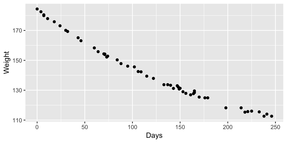
Example: `MASS::wtloss`

The data frame gives the weight, in kilograms, of an obese patient at 52 time points over an 8 month period of a weight rehabilitation programme.

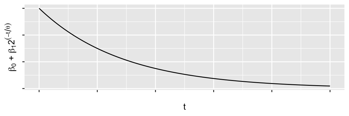
Example: A potential model

\[ y_t = \beta_0 + \beta_1 2^{-t/\theta} + \epsilon_t \] \(\beta_0\), \(\beta_1\) are linear parameters, \(\theta\) is a non-linear parameter.

Your turn

When \(t = 0\), what is \(\E{y_i}\)?
When \(t = \infty\), what is \(\E{y_i}\)?
If \(\E{y_i} = \beta_0 + \tfrac{1}{2}\beta_1\), what is \(t\)?

Fitting non-linear models

Under the Normal error assumption, the MLE of \(\pmb{\beta}\), minimizes \[ \sum_{i = 1}^n (y_i - \eta(\mathbf{x_i}, \pmb{\beta}))^2 \] (the sum of squared residuals) a.k.a non-linear least squares.

There isn’t in general a closed form solution, so iterative procedures are used.
This means you need to provide starting values from the parameters and check that the procedure converged.

Your turn

What might be reasonable values for \(\beta_0\), \(\beta_1\) and \(\theta\)?

In R: `nls()`

wtloss.st <- c(b0 = 100, b1 = 80, th = 100)
fit_nls <- nls(Weight ~ b0 + b1*2^(-Days/th),
  data = wtloss, start = wtloss.st)
fit_nls

## Nonlinear regression model
##   model: Weight ~ b0 + b1 * 2^(-Days/th)
##    data: wtloss
##     b0     b1     th 
##  81.37 102.68 141.91 
##  residual sum-of-squares: 39.24
## 
## Number of iterations to convergence: 4 
## Achieved convergence tolerance: 5.259e-08

summary(fit_nls)

## 
## Formula: Weight ~ b0 + b1 * 2^(-Days/th)
## 
## Parameters:
##    Estimate Std. Error t value Pr(>|t|)    
## b0   81.374      2.269   35.86   <2e-16 ***
## b1  102.684      2.083   49.30   <2e-16 ***
## th  141.910      5.295   26.80   <2e-16 ***
## ---
## Signif. codes:  0 '***' 0.001 '**' 0.01 '*' 0.05 '.' 0.1 ' ' 1
## 
## Residual standard error: 0.8949 on 49 degrees of freedom
## 
## Number of iterations to convergence: 4 
## Achieved convergence tolerance: 5.259e-08

ggplot(wtloss, aes(Days, Weight)) +
  geom_line(aes(y = fitted(fit_nls)))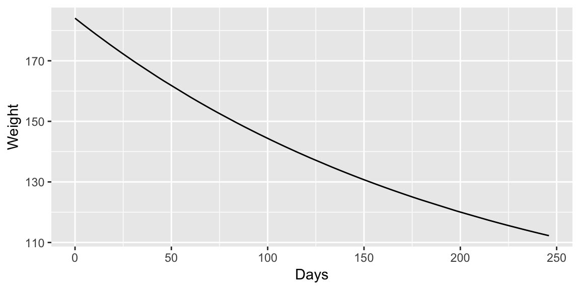

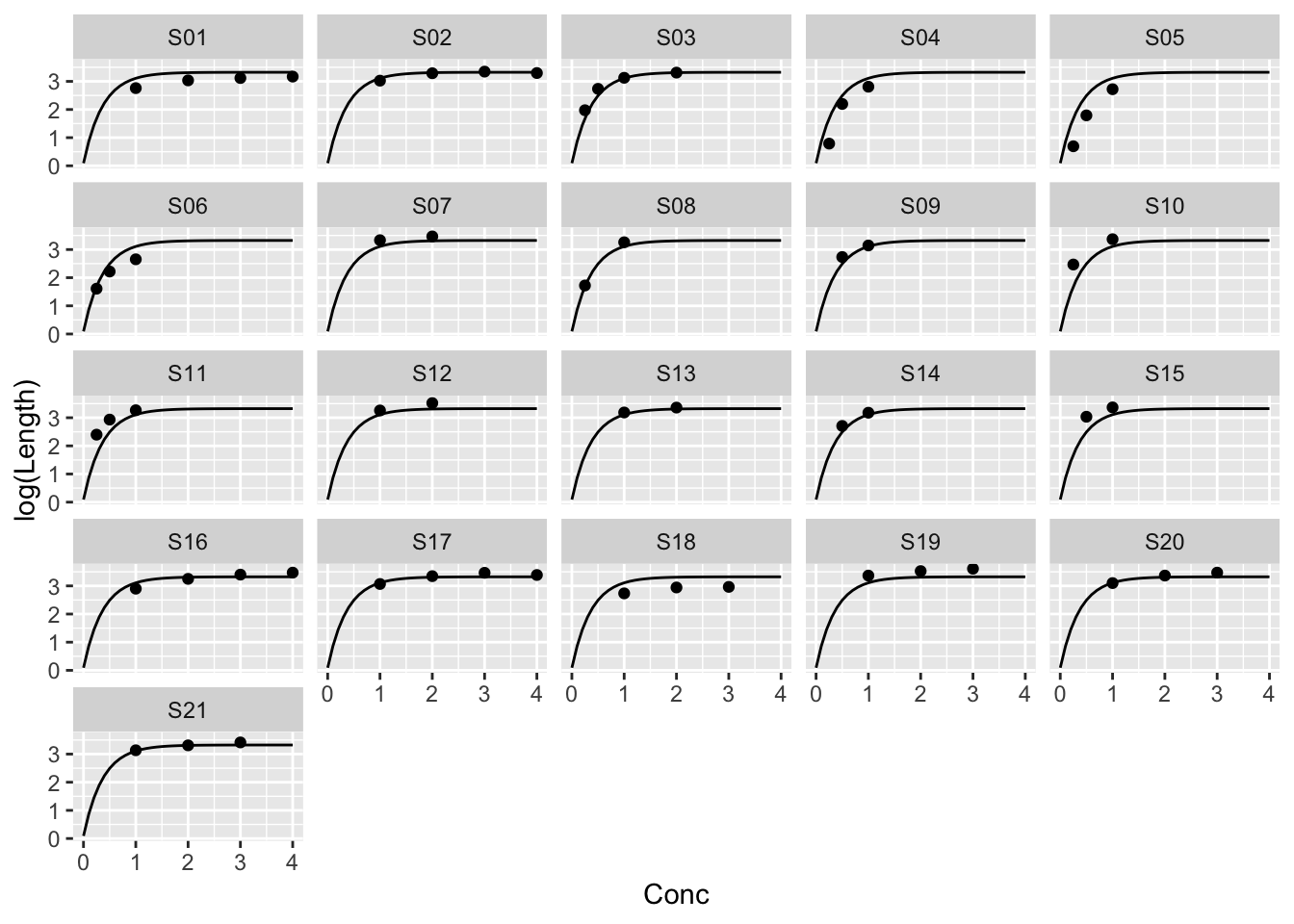
Example: `MASS::muscle`

The purpose of this experiment was to assess the influence of calcium in solution on the contraction of heart muscle in rats. The left auricle of 21 rat hearts was isolated and on several occasions a constant-length strip of tissue was electrically stimulated and dipped into various concentrations of calcium chloride solution, after which the shortening of the strip was accurately measured as the response.

	Strip	Conc	Length
3	S01	1	15.8
4	S01	2	20.8
5	S01	3	22.6
6	S01	4	23.8
9	S02	1	20.6
10	S02	2	26.8

Example: `MASS::muscle`

ggplot(muscle, aes(Conc, log(Length))) + 
  geom_point() + 
  facet_wrap(~ Strip)

Example: The same parameters for every strip

\[ \log{y_{ij}} = \alpha + \beta \rho^{x_{ij}} + \epsilon_{ij} \] \(j\) indexes Strip, \(i\) the ith measurement on a strip.

fit_all <- nls(log(Length) ~ cbind(1, rho^Conc), muscle,
  start = list(rho = 0.05), algorithm = "plinear")

pred_grid <- with(muscle, expand.grid(Conc = seq(0, 4, 0.1),
  Strip = unique(Strip)))
pred_grid$fit_all <- predict(fit_all, pred_grid)

The plinear algorithm takes advantage of the linear parameters.

Example: The same parameters for every strip

Example: Different parameters for every strip

\[ \log{y_{ij}} = \alpha_j + \beta_j \rho^{x_{ij}} + \epsilon_{ij} \]

fit_each <- nls(log(Length) ~ alpha[Strip] + beta[Strip] * rho^Conc,
  muscle,
  start = list(rho = coef(fit_all)[1], alpha = rep(coef(fit_all)[2], 21),
    beta = rep(coef(fit_all)[3], 21)))

pred_grid$fit_each <- predict(fit_each, pred_grid)

Non-linear regression Mar 11 2019

Announcements