What to expect on the final?
- Study guide posted along with last year’s final.
Three questions worth roughly equal amounts
Calculations, inference and interpretation. Like Q2 and Q3 on midterm: t-tests, F-tests, confidence intervals, prediction intervals etc. Know your formulas, how to use them and how to interpret the results.
Assumptions and diagnostics. Examine plots, identify problems, discuss the consequences of the problem, suggest remedies, suggest ways to verify if the suggestions worked. Or suggest ways to diagnose certain problems.
Everything else, at a conceptual level.
Lab in Week 10
Some options:
- Revisit a topic (or more depth on a topic). Which topic?
- Exam review session
- No lab
Today
- The Bias-Variance tradeoff
- Regularized regression: lasso and ridge
Bias-Variance tradeoff
For estimates, the mean squared error of an estimate can be broken down into bias and variance terms: \[ \begin{aligned} MSE(\hat{\theta}) & = \E{(\hat{\theta} - \theta)^2} = \E{\left(\hat{\theta} - \E{\hat{\theta}}\right)^2} + \left(\E{\hat{\theta}} - \theta\right)^2 \\ & = \Var{\hat{\theta}} + \text{Bias}\left(\hat{\theta}\right)^2 \end{aligned} \]
Often in statistics, we focus on estimates that are unbiased (so the second term is zero), and focus on minimising the variance term.
You might argue that you are willing to introduce a little bias, if it reduces the variance enough to reduce the overall mean squared error in the estimate.
There is a similar breakdown for the mean square error in prediction. Let \(\hat{f}(X)\) indicate the regression model for predicting an observation with explanantory values \(X\).
If the true data is generated according to \(Y = f(X) + \epsilon\), where \(\E{\epsilon} = 0\) and \(\Var{\epsilon}= \sigma^2\), then the MSE for a point \(x_0\): \[ \begin{aligned} &MSE(\hat{f}(X)| X = x_0) = \\ \quad &\E{(Y - \hat{f}(X))^2 | X = x_0} \\ \quad &= \E{\left(\hat{f}(x_0) - \E{\hat{f}(x_0)}\right)^2} + \E{\left(Y - \E{\hat{f}(x_0)}\right)}^2 \\ \quad &= \Var{\hat{f}(x_0)} + \text{Bias}\left(\hat{f}(x_0)^2\right) + \sigma^2 \end{aligned} \]
Bias captures how far our predictions are from the true mean on average (over repeated samples).
Variance captures how much our predictions vary (over repeated samples).
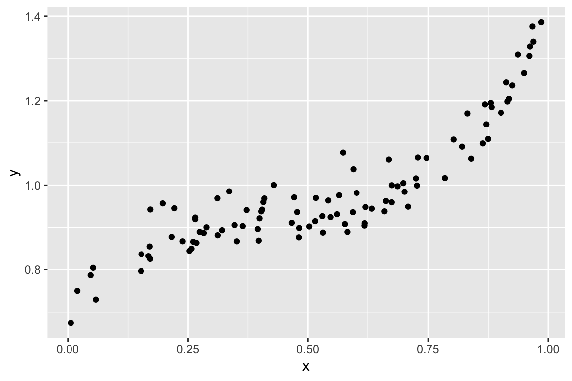
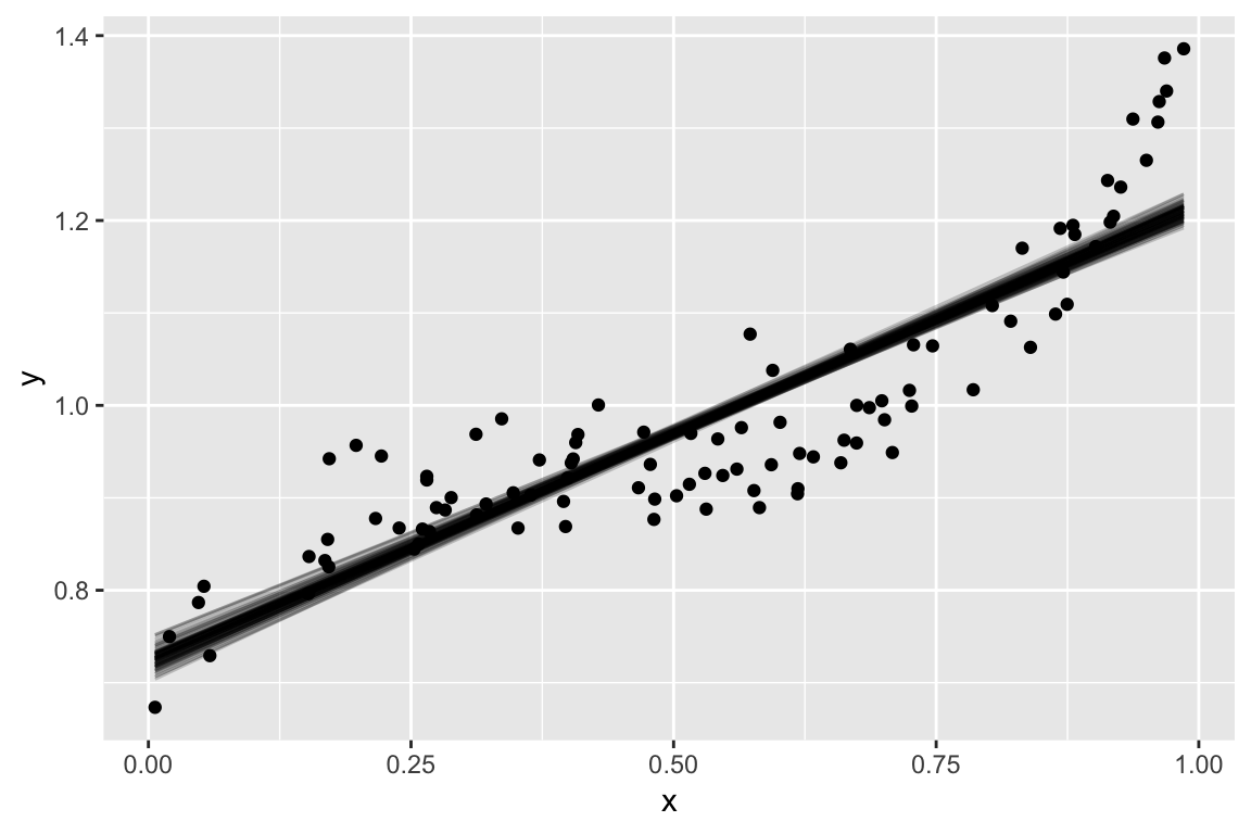
Simulated Example
High bias, low variance
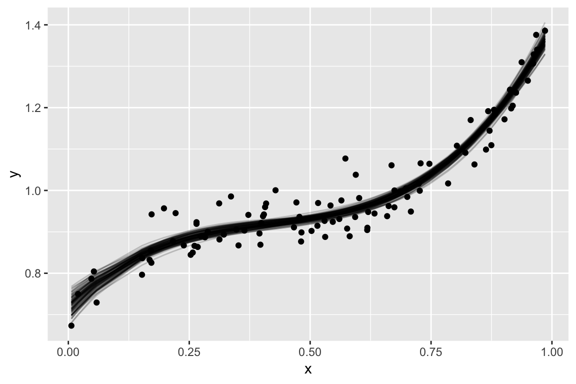
Low bias, low variance
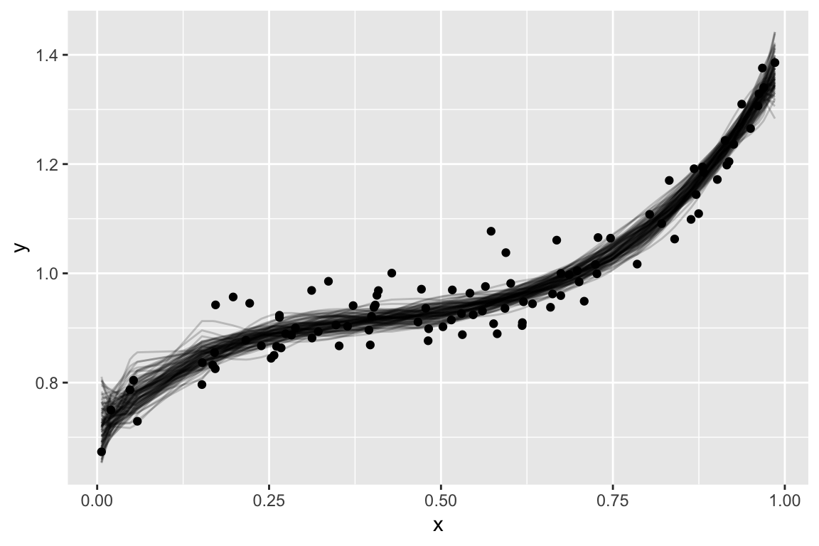
Low bias, high variance
Bias Variance tradeoff
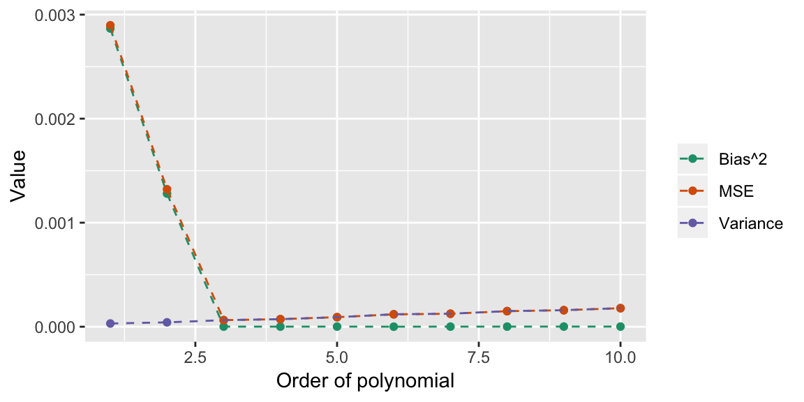
In general, more complex models decrease bias and increase variance. We hunt for the sweet spot where MSE is minimized.
There aren’t nice partitions into bias and variance for other metrics, but the pattern is usually the same. Increasing complexity only improves performance to a point, then it decreases performance.
Regularized regression
One approach that introduces bias into the coefficient estimates, is regularized (a.k.a. penalized) regression. Instead of minimising \[ \sum_{i = 1}^n \left(y_i - \hat{y_i}\right)^2 \] minimise \[ \sum_{i = 1}^n \left(y_i - \hat{y_i}\right)^2 + \lambda \sum_{j = 1}^{p} f(\beta_j) \] When \(f(\beta_j) = \beta_j^2\), the method is called ridge regression, and when \(f(\beta_j) = |\beta_j|\) the method is called lasso.
The general idea: the first term rewards good fit to the data, the second penalizses for large values on the coefficients.
The result: estimates shrink toward zero (introducing bias) and have smaller variance.
Alternative view
You can also view ridge and lasso as constrained minimisation, where we minimise \[ \sum_{i = 1}^n \left(y_i - \hat{y_i}\right)^2 \] subject to the constraints \[ \begin{aligned} \sum_{j = 1}^{p} \beta_j^2 \le t \quad \text{for ridge} \\ \sum_{j = 1}^{p} |\beta_j| \le s \quad \text{for lasso} \end{aligned} \]
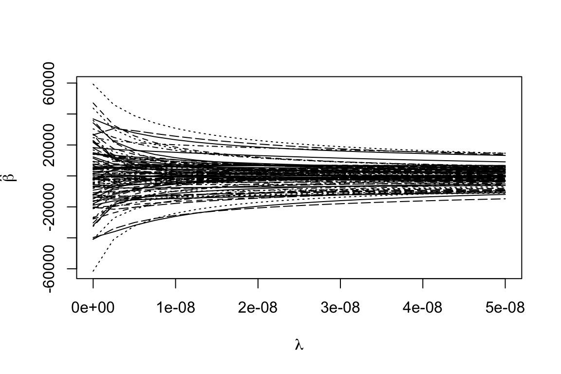
Ridge estimates
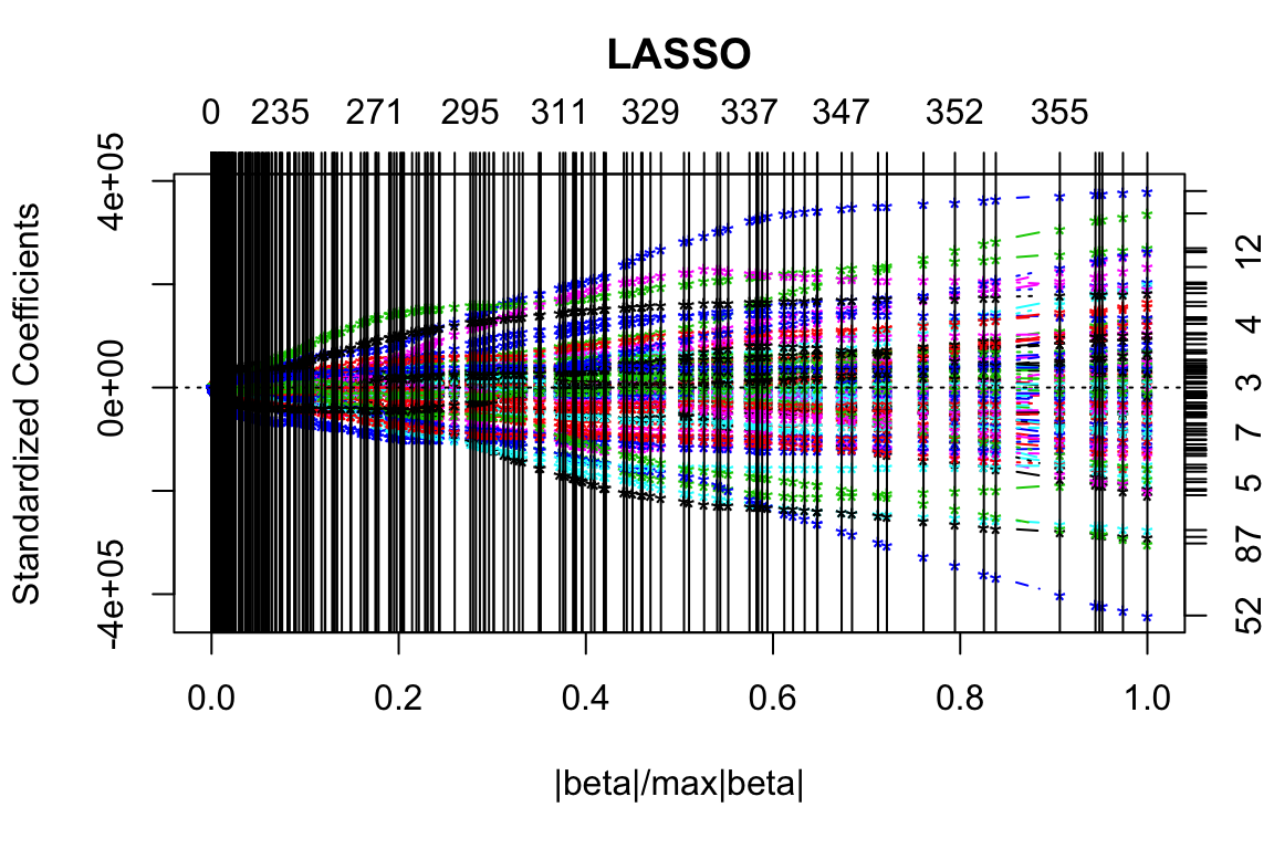
Lasso estimates
Finding the tuning parameter
cvout <- cv.lars(as.matrix(trainmeat[ , -101]), trainmeat$fat)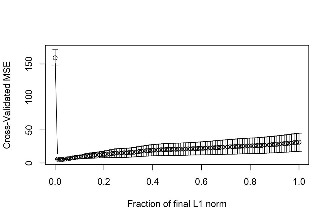
Tuning parameter
(best_s <- cvout$index[which.min(cvout$cv)])## [1] 0.02020202RMSE for this value:
testx <- as.matrix(testmeat[,-101])

predlars <- predict(fit_lasso, testx, s=best_s,
  mode="fraction")
sqrt(mean((testmeat$fat - predlars$fit)^2))
## [1] 2.062124Estimated coefficicents
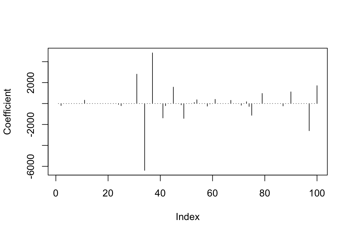
## [1] 27Key points
- Regularized/Penalized regression models have a tuning parameter that controls the degree of penalization/shrinkage
- The tuning parameter may be chosen to optimize some kind of criterion
- Lasso estimates can be exactly zero (so it performs model selection as well)