Transforming the response

In general, transformations make interpretation harder.

We usually want to make statements about the response (not the transformed) response.

Predicted values are easily back-transformed, as well as the endpoints of confidence intervals.

Parameters often do not have nice interpretations on the backtransformed scale.

Special case: Log transformed response

Our fitted model on the transformed scale, predicts: $$\widehat{\log y_i}={\hat{\beta }}_0+{\hat{\beta }}_1{x}_{i1}+\dots +{\hat{\beta }}_p{x}_{ip}$$ If we backtransform, by taking exponential of both sides, $$\widehat{y_i}=\exp {\hat{\beta }}_0\exp \left({\hat{\beta }}_1{x}_{i1}\right)\dots \exp \left({\hat{\beta }}_p{x}_{ip}\right)$$

So, an increase in $x_1$ of one unit, will result in the predicted response being multiplied by $exp\left({\beta }_1\right)$.

If we are willing to assume that on the transformed scale the distribution of the response is symmetric, $$\text{Median}\left(log\left(Y\right)\right)=\text{E}\left(log\right(Y\left)\right)={\beta }_0+{\beta }_1{x}_1+\dots +{\beta }_p{x}_p$$ and back-transforming gives, $$\exp \left(\text{Median}\right(log\left(Y\right)\left)\right)=\text{Median}\left(Y\right)=\exp \left({\beta }_0\right)\exp \left({\beta }_1{x}_1\right)\dots \exp \left({\beta }_p{x}_p\right)$$

So, an increase in $x_1$ of one unit, will result in the median response being multiplied by $exp\left({\beta }_1\right)$.

(For monotone functions $\text{Median}\left(f\left(Y\right)\right)=f\left(\text{Median}\right(Y\left)\right)$,

but $\text{E}\left(f\left(Y\right)\right)\ne f\left(E\right(Y\left)\right)$ in general)

Example

library(faraway)
data(case0301, package = "Sleuth3")
head(case0301, 2)

##   Rainfall Treatment
## 1   1202.6  Unseeded
## 2    830.1  Unseeded

sumary(lm(log(Rainfall) ~ Treatment, data = case0301))

##                   Estimate Std. Error t value Pr(>|t|)
## (Intercept)        5.13419    0.31787 16.1519  < 2e-16
## TreatmentUnseeded -1.14378    0.44953 -2.5444  0.01408
## 
## n = 52, p = 2, Residual SE = 1.62082, R-Squared = 0.11

It is estimated the median rainfall for unseeded clouds is 0.32 times the median rainfall for seeded clouds.

(Assuming log rainfall is symmetric around its mean)

Box-Cox transformations

Assume, the response is positive, and $$g\left(Y\right)=X\beta +ϵ,ϵ\sim N(0,{\sigma }^{2}I)$$ and that $g$ is of the form $$g_{\lambda }\left(y\right)=\{\begin{array}{cc}\frac{y^{\lambda }-1}{\lambda }& \lambda \ne 0\\ \log \left(y\right)& \lambda =0\end{array}$$

Estimate $\lambda$ with maximum likelihood.

For prediction, pick $\lambda$ as the MLE.

For explanation, pick “nice” $\lambda$ within 95% CI.

Example:

library(MASS)
data(savings, package = "faraway")
lmod <- lm(sr ~ pop15 + pop75 + dpi + ddpi, data = savings)
boxcox(lmod, plotit = TRUE)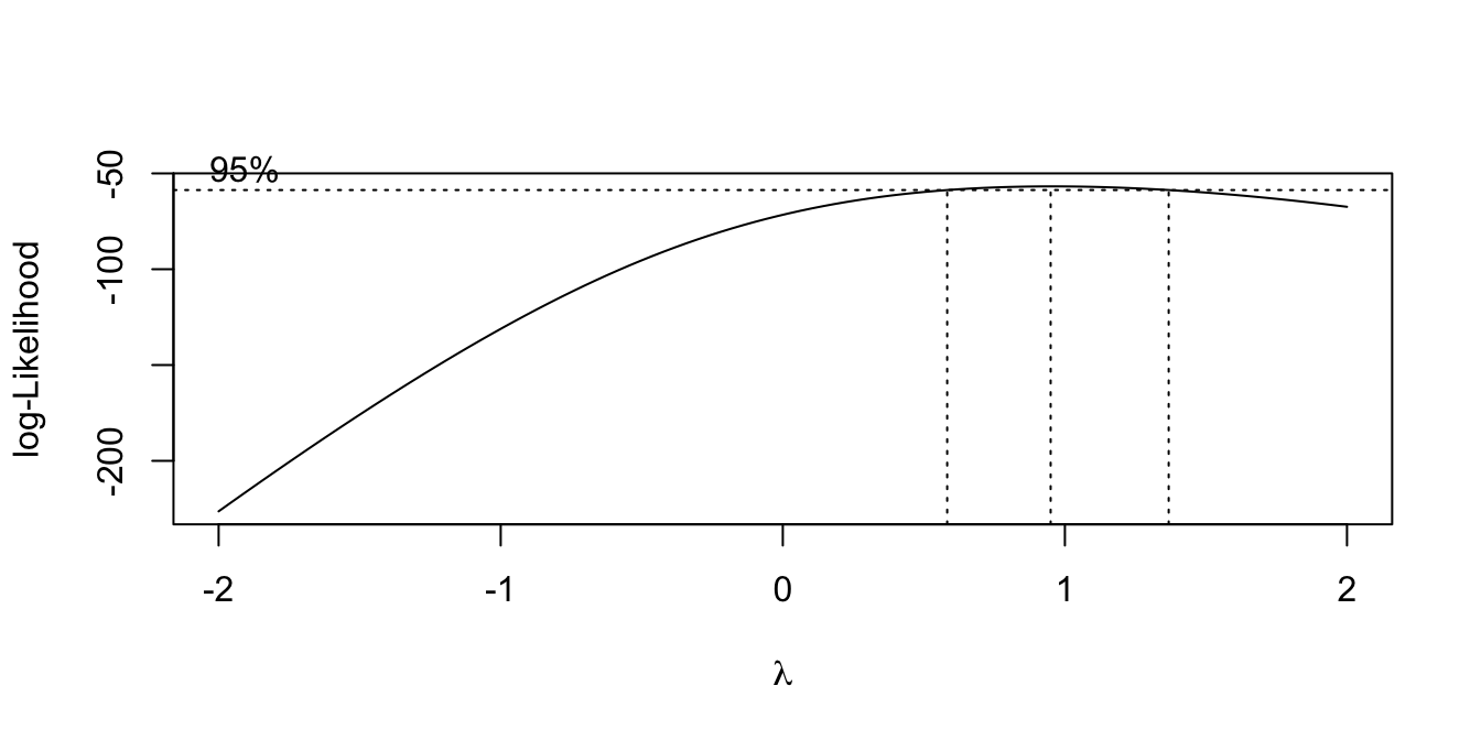

Your turn:

data(gala, package = "faraway")
lmod <- lm(Species ~ Area + Elevation + Nearest + Scruz + Adjacent, 
  data = gala)
boxcox(lmod, plotit = TRUE)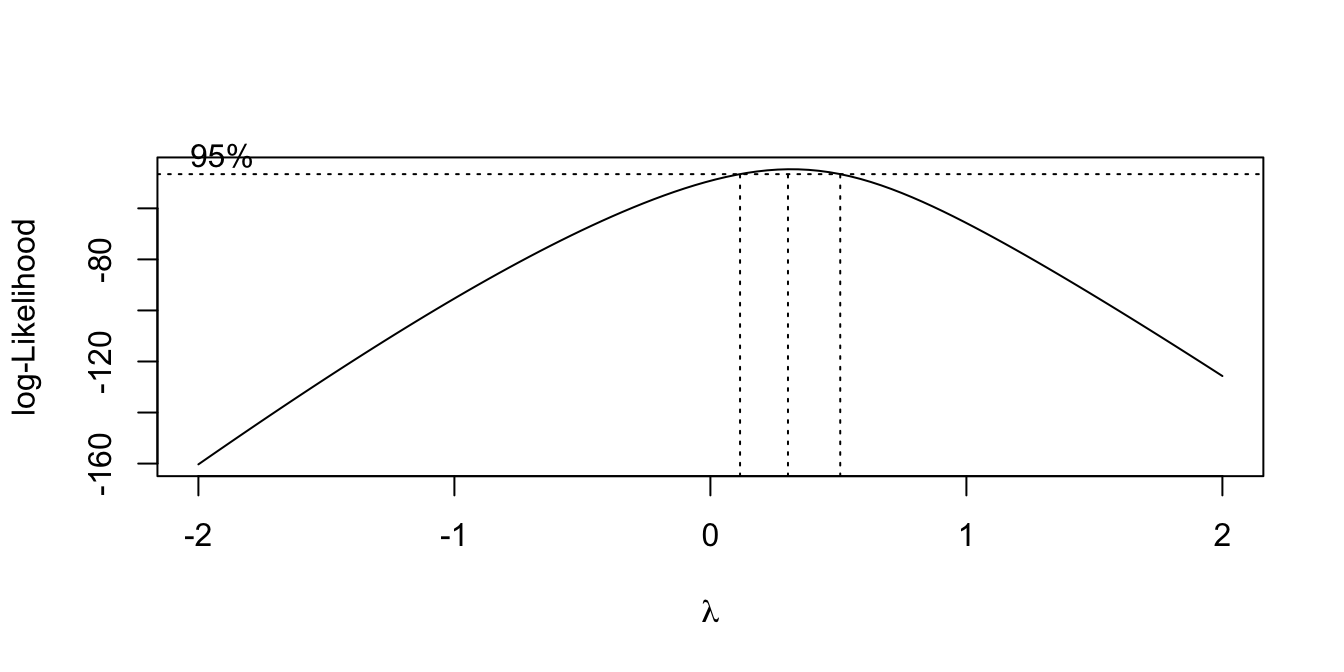

Transforming the predictors

A very general approach is to let the function for each explanatory be represented by a finite set of basis functions. For example, for a single explanatory, X, $$f\left(X\right)=\sum _{k=1}^K{\beta }_k{f}_k\left(X\right)$$ where $f_k$ are the known basis functions, and ${\beta }_k$ the unknown basis coefficients.

Then $$\begin{array}{cc}{y}_i& =f\left(X_i\right)+{ϵ}_i\\ y_i& ={\beta }_1{f}_1\left(X_i\right)+\dots +{\beta }_K{f}_K\left(X_i\right)+{ϵ}_i\\ Y& =X^{\prime }\beta +ϵ\end{array}$$ where the columns of $X^{\prime }$ are $f_1\left(X\right)$, $f_2\left(X\right)$ and we can find the $\beta$ with the usual least squares approach.

Your turn:

What are the columns in the design matrix for the model:

$$y_i={\beta }_{1}1\{X_i<5\}+{\beta }_{2}1\{X_i\ge 5\}+{\beta }_3{X}_{i}1\{X_i<5\}+{\beta }_4{X}_{i}1\{X_i\ge 5\}+{ϵ}_i$$

where $X_i=i,i=1,\dots ,10$?

What do the functions $f_k\left(\right),k=1,\dots ,4$ look like?

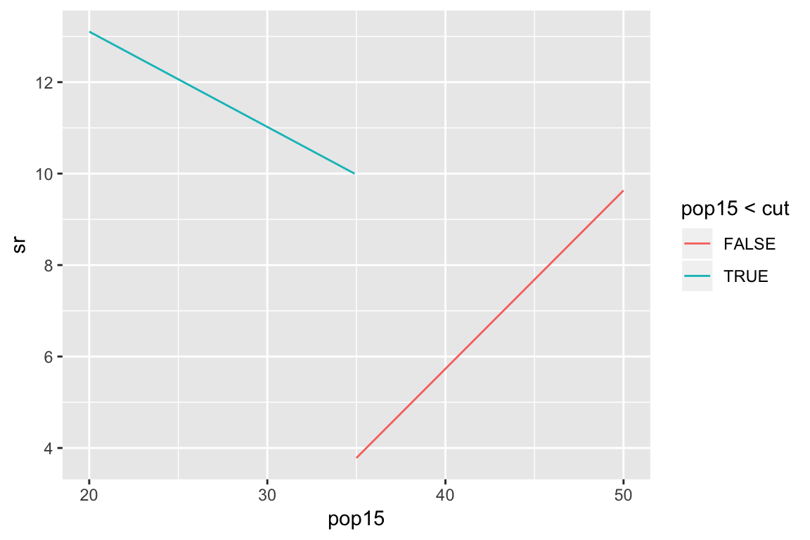
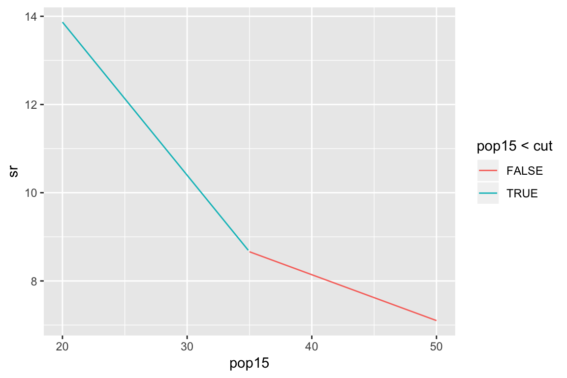
Example: subset regression

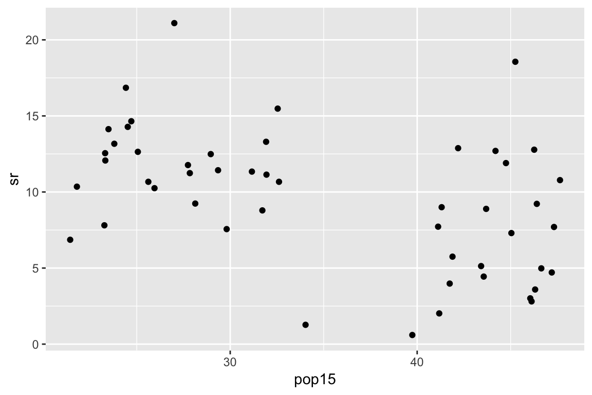
Example: subset regression

cut <- 35
X <- with(savings, cbind(
  as.numeric(pop15 < cut), 
  as.numeric(pop15 >= cut),
  pop15 * (pop15 < cut),
  pop15 * (pop15 >= cut)))

lmod <- lm(sr ~ X - 1, 
  data = savings)
summary(lmod)

Example: subset regression

Broken stick regression

Broken stick:

$$f_1\left(x\right)=\{\begin{array}{cc}c-x& \text{if}x<c\\ 0& \text{otherwise}\end{array}$$ $$f_2\left(x\right)=\{\begin{array}{cc}0& \text{if}x<c\\ x-c& \text{otherwise}\end{array}$$

$$y_i={\beta }_0+{\beta }_1{f}_1\left(X_i\right)+{\beta }_2{f}_2\left(X_i\right)+{ϵ}_i$$

Example: broken stick regression

Polynomials

• Polynomials: $$f_k\left(x\right)=x^k,k=1,\dots ,K$$

• Orthogonal polynomials

• Response surface, of degree $d$ $$f_{kl}(x,z)=x^k{z}^l,k,l\ge 0\text{s.t.}k+l=d$$

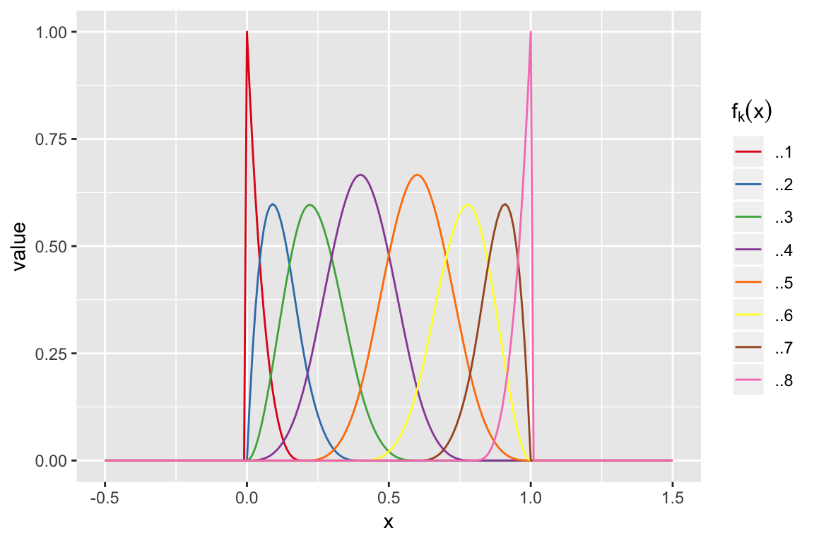
Cubic Splines

Knots: 0, 0, 0, 0, 0.2, 0.4, 0.6, 0.8, 1, 1, 1 and 1

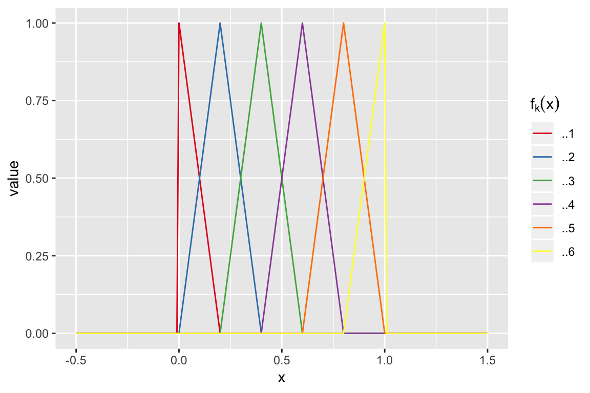
Linear splines

Knots: 0, 0, 0.2, 0.4, 0.6, 0.8, 1 and 1

In practice splines provide a flexible fit

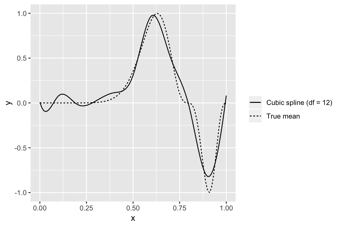
• Smoothing splines: have a large set of basis functions, but penalize against wiggliness

• Generalized Additive Models: simultaneously estimate

$$y_i=f\left(x_{i1}\right)+g\left(x_{i2}\right)+\dots +{ϵ}_i$$

Transforming predictors with basis functions

• The parameters in these regressions no longer have nice interpretations. The best way to present the results is a plot of the estimated function for each X, (or surfaces if variables interact),

• The significance of a variable can still be assessed with an Extra Sum of Squares F-test, comparing to a model without any of the terms relating to a particular variable.