Problems with the error Feb 22 2019

Today

Problems with the errors

• Generalized Least Squares
• Lack of fit F-tests
• Robust regression

Generalized Least Squares

$$Y=X\beta +ϵ$$

• We have assumed $\text{Var}\left(ϵ\right)={\sigma }^{2}I$, but what if we know $\text{Var}\left(ϵ\right)={\sigma }^2\Sigma$, where ${\sigma }^2$ is unknown, but $\Sigma$ is known. For example, we know the form of the correlation and/or non-constant variance in the response.

• The usual least squares estimates ${\hat{\beta }}_{LS}$ are unbiased, but they are no longer BLUE.

Let $S$ be the matrix square root of $\Sigma$, i.e. $\Sigma =S{S}^T$.

Define a new regression equation by multiplying both sides by $S^{-1}$: $$\begin{array}{cc}{S}^{-1}Y& =S^{-1}X\beta +S^{-1}ϵ\\ Y^{\prime }& =X^{\prime }\beta +{ϵ}^{\prime }\end{array}$$

Your Turn

Show $\text{Var}\left({ϵ}^{\prime }\right)=\text{Var}\left(S^{-1}ϵ\right)={\sigma }^{2}I$.

Show the least squares estimates for the new regression equation reduce to: $$\hat{\beta }=(X^T{\Sigma }^{-1}X{)}^{-1}{X}^T{\Sigma }^{-1}Y$$

• Can also show $\text{Var}\left(\beta \right)=(X^T{\Sigma }^{-1}X{)}^{-1}{\sigma }^2$.

• The estimates: $\hat{\beta }=(X^T{\Sigma }^{-1}X{)}^{-1}{X}^T{\Sigma }^{-1}Y$ are known as estimates.

• In practice, $\Sigma$ might only be know up to a few parameters that also need to be estimated.

Common cases of GLS

• $\Sigma$ defines a temporal or spatial correlation structure
• $\Sigma$ defines a grouping structure
• $\Sigma$ is diagonal and defines a weighting structure ()

In R

?lm # use weights argument
library(nlme)
?gls # has weights and/or correlation argument

Oat yields

Data from an experiment to compare 8 varieties of oats. The growing area was heterogeneous and so was grouped into 5 blocks. Each variety was sown once within each block and the yield in grams per 16ft row was recorded.

$${\text{yield}}_i={\beta }_0+{\beta }_1{\text{variety}}_i+{ϵ}_{i}i=1,\dots ,40$$ $$\text{Var}\left({ϵ}_i\right)={\sigma }^2,\text{Cor}({ϵ}_i,{ϵ}_j)=\{\begin{array}{cc}\rho ,& {\text{block}}_i={\text{if block}}_j\\ 0,& \text{otherwise}\end{array}$$

library(nlme) 
fit_gls <- gls(yield ~ variety, data = oatvar, 
  correlation = corCompSymm(form = ~ 1 | block))

Oat yields in R

intervals(fit_gls)

## Approximate 95% confidence intervals
## 
##  Coefficients:
##                  lower  est.       upper
## (Intercept) 291.542999 334.4 377.2570009
## variety2     -4.903898  42.2  89.3038984
## variety3    -18.903898  28.2  75.3038984
## variety4    -94.703898 -47.6  -0.4961016
## variety5     57.896102 105.0 152.1038984
## variety6    -50.903898  -3.8  43.3038984
## variety7    -63.103898 -16.0  31.1038984
## variety8      2.696102  49.8  96.9038984
## attr(,"label")
## [1] "Coefficients:"
## 
##  Correlation structure:
##          lower      est.     upper
## Rho 0.06596382 0.3959955 0.7493731
## attr(,"label")
## [1] "Correlation structure:"
## 
##  Residual standard error:
##    lower     est.    upper 
## 33.39319 47.04679 66.28298

Lack of fit F-tests

• $\widehat{{\sigma }^2}$ should be (if our model is specified correctly) an unbiased estimate of ${\sigma }^2$.

• A “model free” estimate of ${\sigma }^2$ is available if there are replicates (multiple observations at combinations of the explanatory values).

• If our $\widehat{{\sigma }^2}$ from our model is much bigger than the “model-free” estimate, we have evidence of .

In practice

• Fit a saturated model. Compare saturated model to proposed model with an F-test. .

• Saturated: every combination of explanatory variables is allowed its own mean (i.e. every group of replicates is allowed its own mean). A model that includes every explantory as categorical and every possible interaction between variables.

Example

data(corrosion, package = "faraway")
lm_cor <- lm(loss ~ Fe, data = corrosion)
lm_sat <- lm(loss ~ factor(Fe), data = corrosion)
anova(lm_cor, lm_sat)

## Analysis of Variance Table
## 
## Model 1: loss ~ Fe
## Model 2: loss ~ factor(Fe)
##   Res.Df     RSS Df Sum of Sq      F   Pr(>F)   
## 1     11 102.850                                
## 2      6  11.782  5    91.069 9.2756 0.008623 **
## ---
## Signif. codes:  0 '***' 0.001 '**' 0.01 '*' 0.05 '.' 0.1 ' ' 1

# significant lack of fit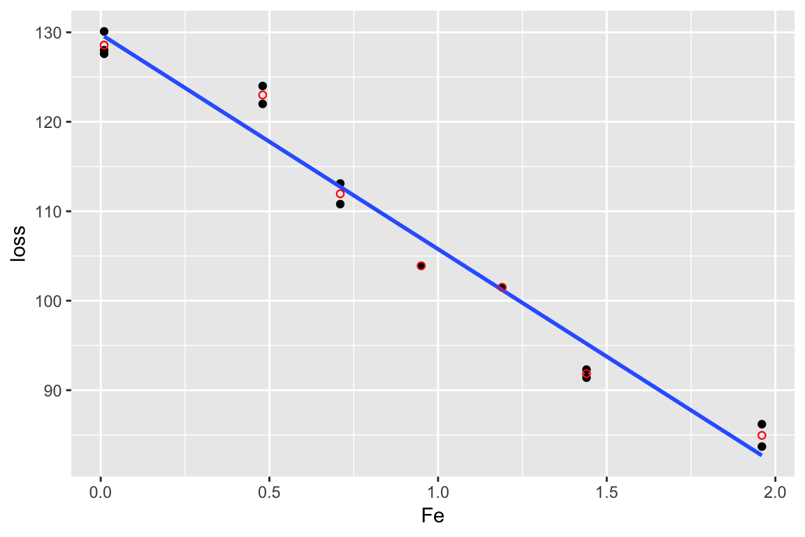

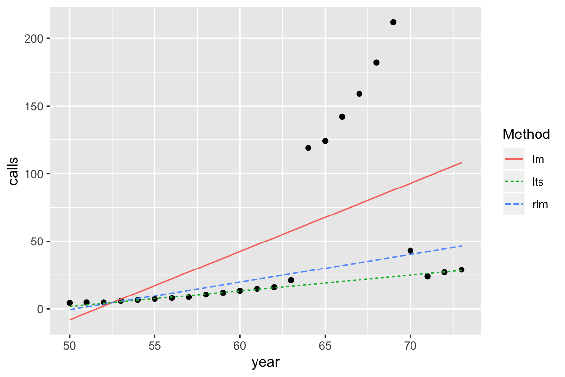
Robust regression

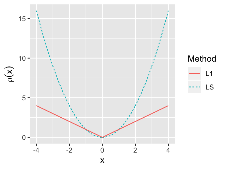
Remember to define our least squares estimates we looked for $\beta$ to minimise $$\sum _{i=1}^n{(y_i-x_i^T\beta )}^2$$

In practice, since we are squaring residuals, observations with large residuals carry a lot of weight. For, robust regression, we want to downweight the observations with large residuals.

The idea of M-estimators is to extend this to the general situation where we want to find $\beta$ to minimise $$\sum _{i=1}^n\rho (y_i-x_i^T\beta )$$ where $\rho \left(\right)$ is some function we specify.

$$\sum _{i=1}^n\rho (y_i-x_i^T\beta )$$

• Least squares: $\rho \left(e_i\right)=e_i^2$
• Least absolute deviation, L${}_1$ regression: $\rho \left(e_i\right)=|e_i|$
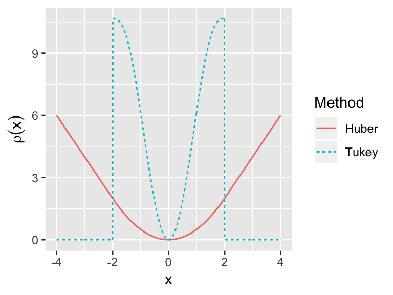
• Huber’s method $$\rho \left(e_i\right)=\{\begin{array}{cc}{e}_i^2/2& \text{if}|e_i|\le c\\ c|e_i|-c^2/2& \text{otherwise}\end{array}$$
• Tukey’s bisquare $$\rho \left(e_i\right)=\{\begin{array}{cc}\frac{1}{6}(c^6-(c^2-e_i^2{)}^3)& |e_i|\le c\\ 0& \text{otherwise}\end{array}$$

The models are usually fit in an iterative process.

Least trimmed squares

Minimise the smallest residuals $$\sum _{i=1}^q{e}_{\left(i\right)}^2$$ where $q$ is some number smaller than $n$ and $e_{\left(i\right)}$ is the ith smallest residual.

One choice, $q=\lfloor n/2\rfloor +\lfloor (p+1)/2\rfloor$

Annual numbers of telephone calls in Belgium