Problems with predictors Feb 20 2019

Roadmap

Done:

• Regression model set up and assumptions
• Least squares estimates and properties
• Inference
• Diagnostics

To Do:

• Specific problems that arise and some extensions
• Model Selection (week 8)
• Some case studies (week 9)
• Non-linear, binary data (week 10)

There will be 8 homeworks total, recall your lowest score is dropped.

Today

Problems with predictors (Faraway 7)

• Collinearity
• Linear transformations of variables
• Errors in predictors

Seat position in cars

data(seatpos, package = "faraway")
?seatpost

Car drivers like to adjust the seat position for their own comfort. Car designers would find it helpful to know where different drivers will position the seat depending on their size and age. Researchers at the HuMoSim laboratory at the University of Michigan collected data on 38 drivers.

The dataset contains the following variables:

library(ggplot2)
ggplot(seatpos, aes(Ht, hipcenter)) +
  geom_point()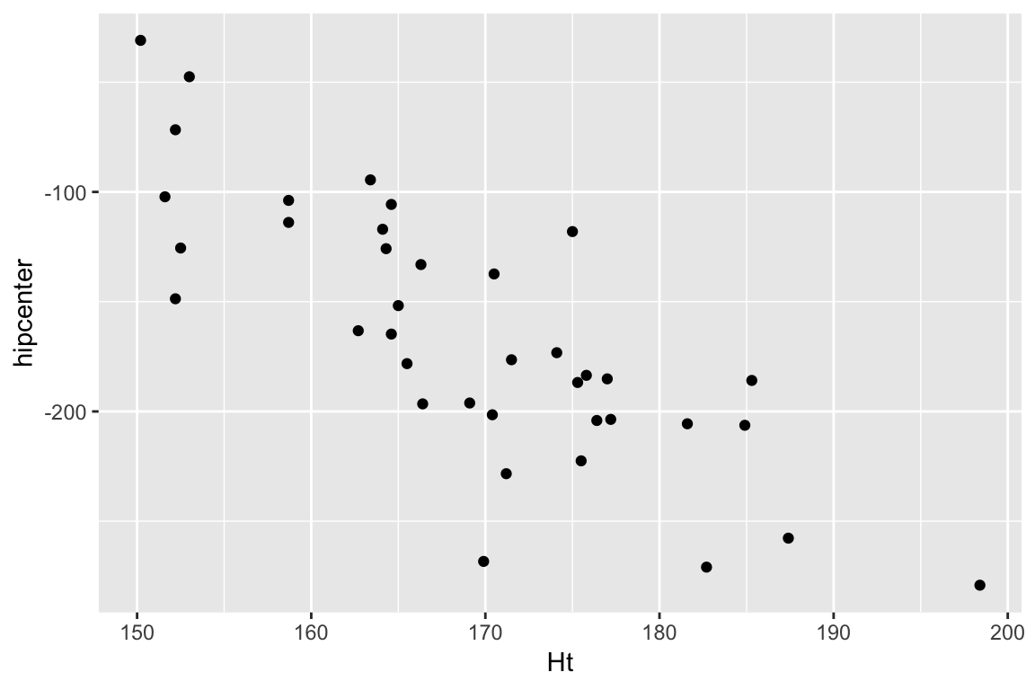

lmod <- lm(hipcenter ~ ., data = seatpos)
sumary(lmod)

##               Estimate Std. Error t value Pr(>|t|)
## (Intercept) 436.432128 166.571619  2.6201  0.01384
## Age           0.775716   0.570329  1.3601  0.18427
## Weight        0.026313   0.330970  0.0795  0.93718
## HtShoes      -2.692408   9.753035 -0.2761  0.78446
## Ht            0.601345  10.129874  0.0594  0.95307
## Seated        0.533752   3.761894  0.1419  0.88815
## Arm          -1.328069   3.900197 -0.3405  0.73592
## Thigh        -1.143119   2.660024 -0.4297  0.67056
## Leg          -6.439046   4.713860 -1.3660  0.18245
## 
## n = 38, p = 9, Residual SE = 37.72029, R-Squared = 0.69

• Exact collinearity If \(X^TX\) is singular, we say there is exact collinearity. There is at least one column that is a linear combination of the others. In R you will get NA for some estimates. Solution drop a column involved, or add constraints on the parameters

• Collinearity or multi-collinearity refers to the case where \(X^TX\) is close to singular. There is at least one column that is almost a linear combination of the others. Or in other words one column is highly correlated with a combination of others.

  In practice this leads to imprecise estimates (i.e. estimates with large standard errors)

Variance inflation factors

Let \(R_i^2\) be the \(R^2\) from the regression of the \(i\)th explanatory variable on all the other explanatory variables. That is, the proportion of the variation in the \(i\)th explanatory variable that is explained by the other explanatory variables.

If the \(i\)th variable was orthogonal to the other variables, \(R_i^2=0\).

If the \(i\)th variable was a linear combination of the other variables, \(R_i^2=1\).

\[ \Var{\hat{\beta_j}} = \sigma^2 \left(\frac{1}{1-R_j^2}\right) \frac{1}{\sum_i (x_{ij} - \bar{x}_j)^2} \] where \(\left(\tfrac{1}{1-R_j^2}\right)\) is known as the variance inflation factor.

This is not a violation of the assumptions

• Multi-collinearity does not violate any regression assumption.

• Our t-tests, F-tests, confidence intervals and prediction intervals all behave as they should.

• The problem is the interpretation of individual parameter estimates. It no longer makes much sense to talk about “… the effect of \(X_1\) holding other variables constant” because we have observed a relationship between \(X_1\) and the other variables.

• We can’t separate the effects of the variables that are collinear, and our standard errors reflect this accurately by being large.

Detecting multicollinearity

In the seat example: large model \(R^2\) but nothing is individually significant. Large standard errors on terms that should be highly significant.

1. Look at the correlation matrix of the explanatory variables. But, this will only identify pairs of explanatories that are correlated (not complicated relationships)
2. Regress \(X_i\) on other variables and look for high \(R^2\), equivalently directly find variance inflation factors.
3. Look at the eigenvalues of \(X^TX\) and look for condition numbers \[ \kappa = \sqrt{\frac{\lambda_1}{\lambda_p}} > 30 \]

Example

Go through example in R

What to do about multicollinearity?

• Most importantly identify when it occurs, so you don’t make stupid statements about individual parameter estimates.

• For prediction, it isn’t a problem as long as future observations have the same structure in the explanatory variables.

• For explanation, we can’t separate the effect of variables that measure the same thing, do joint tests instead.

• Dropping an offending variable is only necessary if you, for some reason, want a model with as few terms as possible. Do not conclude that a variable dropped due to multicollinearity isn’t related to the response!

Errors in variables

We assumed fixed \(X\).

You can also use least squares if \(X\) is random before you observe it, and you want to do inference conditional on the observed \(X\).

If, \(X\) is measured with error, i.e. \[ \begin{aligned} X = X_a + \delta \\ Y = X_a\beta + \epsilon \end{aligned} \] then the least squares estimates will be biased (usually towards zero if \(X_a\) and \(\delta\) are unrelated).

There are “errors in variables” estimation techniques.

Linear transformations of predictors

Transformations of the form \[ X_j \rightarrow \frac{X_j - a}{b} \] do not change the fit of the regression model, only the interpretation of the parameters.

One useful one is to standardise all the explanatory variables \[ X_j \rightarrow \frac{X_j - \bar{X_j}}{s_{X_j}} \] which puts all the parameters on the same scale: “…a change in \(X_j\) of one standard deviation is associated with a change in response of \(\beta_j\)…”

Also, can be useful to re-express a predictor in more reasonable units. For example, expressing income in $1000s rather than $1s.