Case Influence Statistics
A selection of metrics for observations that help identify unusual observations.
Three kinds of unusual observations:
- High leverage observations are unusual in their combination of explanatory values and have the potential to be influential.
- Outliers don’t fit the model well (their combination of response and explanatories is unusual according to the model)
- Influential observations substantially change the model when included/excluded. We don’t want out conclusions to rely heavily on a few influential observations. Generally are also one of high leverage and/or outliers.
Case Influence Statistics
There are many metrics. We’ll cover one for each kind of unusual observation but be aware there are others.
Don’t worry about the formulas, concentrate on the concept. Faraway 6.2
Leverage
The leverage of a observation is \(h_i = H_{ii}\) the \(i\)th diagonal element of the hat matrix, H.
Remember the hat matrix only depends on \(X\).
\(h_i\) is a Mahalanobis distance (wikipedia it).
It’s a measure of how far the observations explanatory values are from the mean of the observed explanatory values, but it takes into account the unequal variances of each explanatory variable and their correlations.
The regression line/surface is pulled towards observations with high leverage.
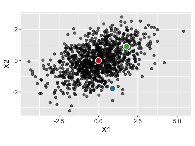
Blue point is much further from the mean in the Mahalanobis sense than the green point. The blue point would have higher leverage.
Outliers
A observation that doesn’t fit the regression model will have a large error, but this doesn’t necessary translate to a large residual because we fit the model to minimize residuals.
Instead of just looking for large residuals, compare the predicted response from a model without the observation (so it can’t influence the model), to the observed response, \[ \hat{y}_{(i)} - y_i \] where \(\hat{y}_{(i)}\) is the fitted value for the \(i\)th observations from a model fitted to the data excluding the \(i\)th observation.
This value, appropriately standardized, is called the Studentized residual.
Influence
How much does the model fit change when the observation is excluded? A substantial change indicates an influential observation. The distance between the vector of fitted values when the ith observation is excluded and fitted values when the ith observation is included is:
\[ (\hat{\mathbf{y}} - \hat{\mathbf{y}}_{(i)})^T (\hat{\mathbf{y}} - \hat{\mathbf{y}}_{(i)}) \]
This value, appropriately scaled, is called Cook’s Distance.
Handout
In each plot:
- Draw in a fitted regression line including the point marked with \(+\), and a fitted regression line excluding the point marked with \(+\)
- Decide if the point marked with \(+\) would be high leverage, an outlier, and/or influential.
Partial plots
Motivation: We can examine a plot of the response against each explanatory, but the observed relationship is complicated by the effect of the other variables.
Useful to graphically check relationships between the response and explanatories after “accounting for” the other variables. Examine for evidence of non-linearity and unusual observations.
Partial regression plots
For explanatory variable, \(j\):
Regress \(y\) on all explanatories except the \(j\)th and find residuals, \(\hat{\delta}\)
Regress \(x_j\) on all explanatories except itself and find residuals, \(\hat{\gamma}\)
Plot \(\hat{\delta}\) against \(\hat{\gamma}\)
Partial residual plots
For explanatory variable, \(j\):
Plot
\[
y_i - \sum_{i\ne j} x_{ij}\hat{\beta}_j
\]
against the \(j\)th explanatory variable.