Randomization Test
The F-tests (and t-tests) rely on the Normal error assumption.
In a randomized experiment, the randomization provides a basis for inference (no i.i.d sampling from populations required) and results in randomization tests.
The same procedure can be used in observational studies, with the assumption that nature ran the experiment for you, i.e. it’s like units were assigned to values of the explanatory variables at random.
Some people call randomization tests used for observational data, permutation tests.
Your Turn
What are the key ingredients in an hypothesis test?
Hypothesis Testing
Randomization Test
(Overall F-test example)
Model: Randomized experiment
Null: Treatments have no effect on response
Test statistic: (Up to us) Let’s use overall regression F-statistic.
Null distribution: Randomization distribution of the test statistic.
The randomized experiment model
\(n\) experimental units \[ u_1 \quad u_2 \quad \ldots \quad u_n \]
\[ X = \begin{pmatrix} 1 & x_{11} & \ldots & x_{1(p-1)} \\ \vdots & \vdots & \ddots & \vdots \\ 1 & x_{n1} & \ldots & x_{n(p-1)} \end{pmatrix} \] \[ y = \begin{pmatrix} y_1 \\ \vdots \\ y_n \end{pmatrix} \] \(y_i\) the observed response for the the unit that was randomly assigned to the \(i\)th row of the design matrix.
Example: Growing tomatoes
\(n\) experimental units
\[ X = \begin{pmatrix} 1 & 1 & 1 \\ 1 & 1 & 0 \\ 1 & 1 & 0 \\ 1 & 0 & 0 \\ 1 & 0 & 1 \\ 1 & 0 & 1 \end{pmatrix} \] \[ y = \begin{pmatrix} 8 \\ 6 \\ 2 \\ 9 \\ 7 \\ 4 \end{pmatrix} \]
Null distribution
If the null is true, treatments have no effect on response.
\[ y = \begin{pmatrix} y_1 \\ \vdots \\ y_n \end{pmatrix} \]
\(y_i\) the observed response for the the unit that was randomly assigned to the \(i\)th row of the design matrix.
If the null is true, I see the same set of \(y_i\), just in different order based on the output of my randomizing units to treatment.
Null distribution: the distribution of the test-statistic for all permutations of \(y_i\)
An equally likely output of the tomato growing experiment
\(n\) experimental units
\[ X = \begin{pmatrix} 1 & 1 & 1 \\ 1 & 1 & 0 \\ 1 & 1 & 0 \\ 1 & 0 & 0 \\ 1 & 0 & 1 \\ 1 & 0 & 1 \end{pmatrix} \] \[ y = \begin{pmatrix} 6 \\ 8 \\ 2 \\ 9 \\ 7 \\ 4 \end{pmatrix} \]
The null distribution
Observed data gives overall F-statistic: 0.132
Equally likely outcomes under the null hypothesis: \[ \begin{pmatrix} 8 \\ 6 \\ 2 \\ 9 \\ 7 \\ 4 \end{pmatrix}, \begin{pmatrix} 6 \\ 8 \\ 2 \\ 9 \\ 7 \\ 4 \end{pmatrix}, \begin{pmatrix} 2 \\ 6 \\ 8 \\ 9 \\ 7 \\ 4 \end{pmatrix}, \begin{pmatrix} 6 \\ 2 \\ 8 \\ 9 \\ 7 \\ 4 \end{pmatrix}, \quad \text{ +716 other possibilities} \]
Equally likely F-statistics under the null hypothesis:
\[ 0.132, \,0.244, \,5.534, \,0.244 \hspace{2in} \]
The null distribution
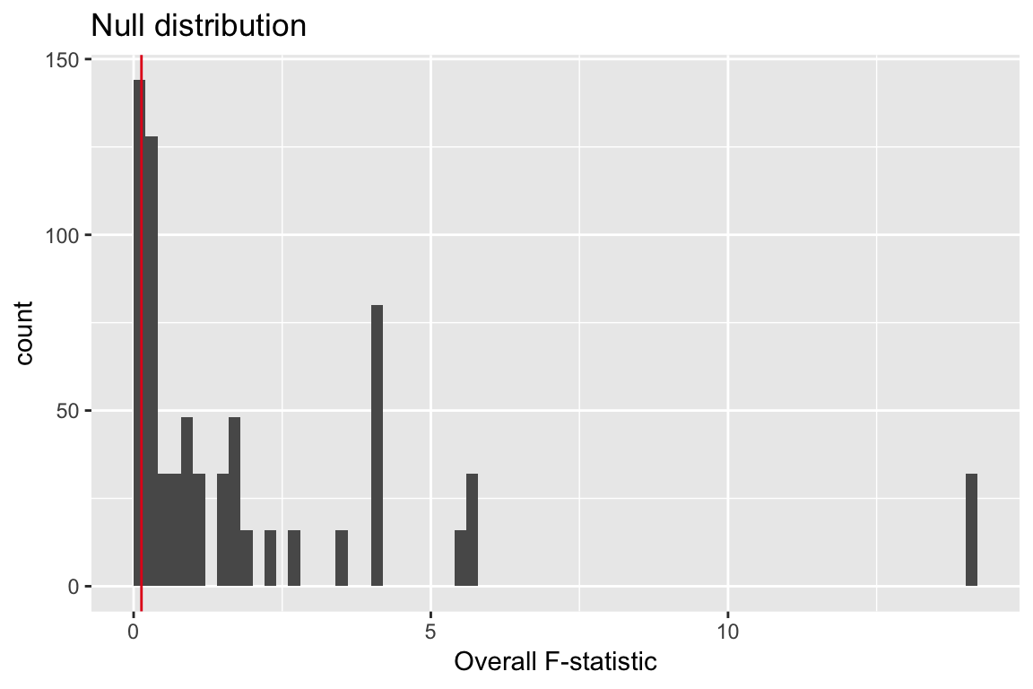
\(624/720 = 0.87\)
Faraway: Galapagos
In lab:
library(faraway)
lmod_small <- lm(Species ~ Nearest + Scruz,
  data = gala)
lms <- summary(lmod_small)
obs_fstat <- lms$fstat[1]

nperms <- 4000
fstats <- numeric(nperms)
for (i in 1:nperms){
  lmods <- lm(sample(Species) ~ Nearest + Scruz,
    data = gala)
  fstats[i] <- summary(lmods)$fstat[1]
}
In practice
Easiest to justify when you actually have a randomized experiment
The choice of test statistic can be important for useful performance and interpretation:
For example, if the treatments affect the variance of the response, not the means, using the overall F-stat may fail to reject the null (treatment has no effect) with high probability even when sample sizes are large.
Sometimes it’s reasonable to add an assumption on the alternative, i.e. treatments have an additive effect.