HW #3 Interpreting \(\hat{\sigma}\)
\(\sigma\) has the same units as the response (\(\sigma^2\) does not).
Could rely on Normal approximation:
We expect roughly 95% of teenagers expenditures on gambling to be within \(\pm\) 45 pounds per year of the mean expenditure based on the regression model.
Or Chebychev:
We expect at least 75% of teenagers expenditures on gambling to be within \(\pm\) 45 pounds per year of the mean expenditure based on the regression model.
Explanation
Sampling
Our model says, we have fixed our \(X\) and our responses are generated according to the model \[ Y = X\beta + \epsilon \quad \epsilon \sim N(0, \sigma^2 I) \] but how does this relate to real life data?
Designed experiments: We fix \(X\) and let nature generate the responses according to the model. We only observe a finite number of observations and our inference tells us about the \(\beta\) underlying the natural generating process.
Observational studies: A population of responses exists for each unique \(X\). We observe a sample from the populations and use our estimate to make inferences on the population value of \(\beta\). Generally, we like simple random samples and sample much smaller than the population (or use finite population corrections).
Sampling cont.
Complete population: Permutation tests give some meaning to the p-value for the sample at hand (more later). Or use regression just as a descriptive tool for the sample at hand. Or imagine parallel alternative worlds.
Random \(X\): some set up regression conditional on \(X\). Can show many of the same properties, i.e. \(E(\hat{\beta} | X) = \beta)\), but must add crucial assumption that \(X\) and \(\epsilon\) are independent.
library(faraway)
data(gala, package = "faraway")
lmod <- lm(Species ~ Area + Elevation + Nearest + Scruz + Adjacent,
  data = gala)
sumary(lmod)
## Estimate Std. Error t value Pr(>|t|)
## (Intercept) 7.068221 19.154198 0.3690 0.7153508
## Area -0.023938 0.022422 -1.0676 0.2963180
## Elevation 0.319465 0.053663 5.9532 3.823e-06
## Nearest 0.009144 1.054136 0.0087 0.9931506
## Scruz -0.240524 0.215402 -1.1166 0.2752082
## Adjacent -0.074805 0.017700 -4.2262 0.0002971
##
## n = 30, p = 6, Residual SE = 60.97519, R-Squared = 0.77What is the meaning of \(\hat{\beta}_\text{Elevation} = 0.32\)?
Naive (wrong) interpretation
A unit increase in \(x_1\) will produce a change of \(\beta_1\) in the response
Where does this come from? Compare \((y_i | X_{i1} = x_1)\) to \((y_i | X_{i1} = x_1 + 1)\)
Or compare \(E(y_i | X_{i1} = x_1)\) to \(E(y_i | X_{i1} = x_1 + 1)\)
A unit increase in \(x_1\) is associated with a change of \(\beta_1\) in the mean response
Compare two islands where the elevation of one island is one meter higher than the first. On average the second island has 0.32 species more than the first.
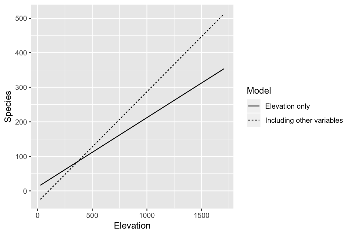
More accurate interpretation
You must be specific about what else is in the model, because the meaning of \(\beta_1\) is different in the following models \[ y_i = \beta_0 + \beta_1 \text{Elevation}_i + \epsilon_i \] \[ y_i = \beta_0 + \beta_1 \text{Elevation}_i + \beta_2 \text{Area}_i + \beta_3 \text{Nearest}_i + \beta_4 \text{Scruz} + \beta_5 \text{Adjacent} + \epsilon_i \]
Better
A unit increase in \(x_1\) with the other (named) predictors held constant is associated with a change of \(\beta_1\) in the response
Compare two islands with the same area, distance to nearest island, distance from Santa Cruz island, and area of the adjacent island, but where the elevation of one island is one meter higher than the first. On average the second island has 0.32 species more than the first.
But these are purely hypothetical islands. We can’t change any of these properties, let alone one without the others.
Causal inference
2008 Democratic primaries in NH
“On the 8th January 2008, primaries to select US presidential candidates were held in New Hampshire. In the Democratic party primary, Hillary Clinton defeated Barack Obama contrary to the expectations pre-election opinion polls. Essentially two different voting technologies were used in New Hampshire. Some wards used paper ballots, counted by hand while others used optically scanned ballots, counted by machine. Among the paper ballots, Obama had more votes than Clinton while Clinton defeated Obama on just the machine counted ballots. Since the method of voting should make no causal difference to the outcome, suspicions have been raised regarding the integrity of the election.” –
?newhamp
2008 Democratic primaries in NH
##              Estimate Std. Error t value  Pr(>|t|)
## (Intercept) 0.3525171  0.0051728 68.1480 < 2.2e-16
## handcount   0.0424871  0.0085091  4.9932 1.059e-06
##
## n = 276, p = 2, Residual SE = 0.06823, R-Squared = 0.08
\[ \text{Proportion for Obama}_i = y_i = \beta_0 + \beta_1 \text{handcount}_i + \epsilon_i \]
What is the meaning of \(\hat{\beta}_1 = 0.04\)?
Your Turn: Indicator Variables
\[ \text{handcount}_i = \begin{cases} 1, & \text{ward i counted votes by hand} \\ 0, & \text{otherwise (ward i counted by machine)} \end{cases} \]
Find \(E(y_i | \text{handcount}_i = 1)\), and \(E(y_i | \text{handcount}_i = 0)\).
What is \(E(y_i | \text{handcount}_i = 1) - E(y_i | \text{handcount}_i = 0)\)?
Explain in words in context of the problem.
Equivalent to an equal variance two sample t-test
t.test(pObama ~ handcount, data = newhamp, var.equal = TRUE)##
## Two Sample t-test
##
## data: pObama by handcount
## t = -4.9932, df = 274, p-value = 1.059e-06
## alternative hypothesis: true difference in means is not equal to 0
## 95 percent confidence interval:
## -0.05923854 -0.02573565
## sample estimates:
## mean in group 0 mean in group 1
## 0.3525171 0.3950042A non-causal conclusion:
The wards with handcounting had on average a proportion of votes for Obama 4 percentage points higher than the wards with digital counts.
Can me make the causal conclusion?
Handcounting increased the proportion of votes for Obama by 4 percentage points.
Causality
A causal effect is the difference between outcomes where action was taken or not.
Let \(T = 1\) for the treatment and \(T = 0\) be the control. Then \(y^1_i\) be the observed response for subject \(i\) under the control and \(y^0_i\) be the observed response for subject \(i\) under the treatment.
We want to know: \[ \delta_ i = y^1_i - y^0_i \]
The fundemental problem: we can only observe one of \((y^1_i, y^0_i)\).
Confounders
Suppose the correct model was \[ \text{Proportion for Obama}_i = \beta^*_0 + \beta^*_1 \text{handcount}_i + \beta^*_2 Z_i + \epsilon_i \] where \(Z\) is some third variable that is related also to our treatment variable: \[ Z_i = \gamma_0 + \gamma_1\text{handcount}_i + \epsilon'_i \]
Our conclusions from our original model would only be accurate if \(\beta^*_2 = 0\), or \(\gamma_1 = 0\).
\(Z\) is known as a confounder.
Ways to proceed
Randomized experiment We control which observation we make. We randomize units to treatments. On average, confounders will be balanced across treatment groups. But, more importantly randomization provides a complete basis for inference about the average treatment effect. Causal inference in justified without further assumptions.
Close substitution We argue that we can observe things that are very close to \(y^1_i\) and \(y^0_i\).
Ways to proceed
Matching We match observations based in similar covariates to provide a fair comparison.
Statistical adjustment We know about confounders and model their effects to remove their contribution.
See Faraway Chapter 5 for covariate adjustment and matching for the voting data.
A real-life example
Do Nike Vaporfly shoes actually make you run faster?
https://www.nytimes.com/interactive/2018/07/18/upshot/nike-vaporfly-shoe-strava.html