Today
- Inference on the coefficients
- F-tests
Inference on the coefficients
With the addition of the Normality assumption,
\[ \frac{\hat{\beta_0} - \beta_0}{\sqrt{\VarH{\hat{\beta_0}}}} \sim t_{n-2} \quad \text{and} \quad \frac{\hat{\beta_1} - \beta_1}{\sqrt{\VarH{\hat{\beta_1}}}} \sim t_{n-2} \] where \(\VarH{.}\) is the variance of the estimate with \(\hat{\sigma}\) plugged in for \(\sigma\).
Leads to confidence intervals and hypothesis tests of the individual coefficients.
Also under Normality the least squares estimates of slope and intercept are the maximum likelihood estimates.
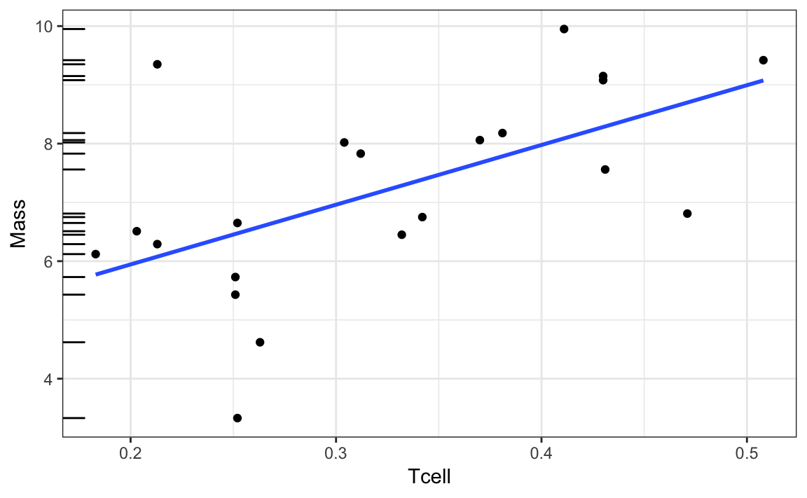
Weightlifting birds
Recall the model: \[ \text{Mass}_i = \beta_0 + \beta_1 \text{Tcell}_i + \epsilon_i, \quad i = 1, \ldots, 21 \]
\(\hat{\beta_1}\) = 10.165
\(\VarH{\hat{\beta_1}} = 3.296^2\)
What’s the t-statistic for testing the null hypothesis \(H_0: \beta_1 = 0\)?
summary(slr)
#>
#> Call:
#> lm(formula = Mass ~ Tcell, data = ex0727)
#>
#> Residuals:
#>     Min      1Q  Median      3Q     Max
#> -3.1429 -0.7327  0.3448  0.7472  3.2736
#>
#> Coefficients:
#>             Estimate Std. Error t value Pr(>|t|)
#> (Intercept)    3.911      1.112   3.517  0.00230 **
#> Tcell         10.165      3.296   3.084  0.00611 **
#> ---
#> Signif. codes:  0 '***' 0.001 '**' 0.01 '*' 0.05 '.' 0.1 ' ' 1
#>
#> Residual standard error: 1.426 on 19 degrees of freedom
#> Multiple R-squared:  0.3336, Adjusted R-squared:  0.2986
#> F-statistic: 9.513 on 1 and 19 DF,  p-value: 0.006105
Prediction
Consider some new observation with explanatory value \(x_0\). The true response is, \[ y_0 = \beta_0 + \beta_1 x_0 + \epsilon \] with expected value \[ \E{y_0} = \beta_0 + \beta_1 x_0 \]
There are two things we might be interested in:
- estimating the mean response at this value, \(\hat{\text{E}}(y_0)\)
- predicting the response at this value, \(\text{Pred}({y_0})\)
For both cases the point prediction is, \[ \text{Pred}({y_0}) = \hat{y_0} = \hat{\beta_0} + \hat{\beta_1} x_0 \]
Confidence interval on the mean response
When estimating the mean response, uncertainty only comes from the uncertainty in our estimates of the slope and intercept.
\[ \Var{\hat{y_0}} = \sigma^2 \left[\frac{1}{n} + \frac{(x_0 - \bar{x})^2}{\sum_{i=1}^n (x_i - \bar{x})^2} \right] \]
Leads to confidence intervals of the form \[ \hat{y_0} \pm t_{n-2, 1 - \alpha/2} \sqrt{\VarH{\hat{y_0}}} \]
“With 95% confidence, we estimate the mean response is between …”
Prediction interval for a new response
When predicting a new response, uncertainty also comes from the variation about the mean.
\[ \Var{\text{Pred}({y_0})} = \Var{\hat{y_0}} + \sigma^2 \]
Leads to prediction intervals of the form \[ \hat{y_0} \pm t_{n-2, 1 - \alpha/2} \sqrt{\VarH{\text{Pred}({y_0})}} \]
“A 95% prediction interval for the response is …”
(I don’t like the wording “With 95% probability, …” because it isn’t quite correct, part of our uncertainty is still uncertainty in the estimation of parameters, not just uncertainty from the random error.)
General Idea: Partitioning the variation
We see variation in the response. We want to attribute that variation to different sources: variation due to the mean varying according to our regression model, and variation due to the random error.
Sketch
Partition of variation
\[ \begin{aligned} \text{Total Sum of Squares} = \sum_{i=1}^n{(y_i - \bar{y})^2} \\ \text{Residual Sum of Squares} = \sum_{i=1}^n{(y_i - \hat{y}_i)^2} \end{aligned} \]
Can show \[ \begin{aligned} \sum_{i=1}^n{(y_i - \bar{y})^2} &= \sum_{i=1}^n{(y_i - \hat{y}_i)^2} &+& \sum_{i=1}^n{(\hat{y}_i - \bar{y})^2} \\ \text{Total SS} &= \text{Residual SS} &+& \text{Regression SS} \end{aligned} \] Many notations:
Total SS = TSS = \(SS_{Total}\) = \(SS(Total)\)
Residual SS = RSS = SSE = \(SS_{Res}\) = \(SS(Res)\)
Regression SS = SSR = \(SS_{Reg}\) = \(SS(Reg)\) = \(SS(Model)\)
Degrees of freedom
The degrees of freedom for each sum of squares are also additive \[ \begin{aligned} n-1 &= n-2 &+& 1 \\ \text{Total df} &= \text{Residual d.f.} &+& \text{Regression d.f.} \end{aligned} \]
\(\text{SS}(.) / \text{d.f.}(.) = \text{Mean sum of squares} (.) = \text{MSS}(.)\)
R-squared
\(R^2\) is simply the proportion of variation in the response explained by the model
\[ R^2 = \frac{\text{Total SS} - \text{Residual SS}}{\text{Total SS}} \]
In simple linear regression \(R^2\) is the square of the Pearson correlation between \(x\) and \(y\).
Next Week
I’m out of town, Trevor, your TA, will lead lecture and lab.
I’ll be reachable by email, but will have limited time to respond, especially on Tue and Wed.
You don’t need to print the notes, Trevor will bring a packet for the week for you on Monday (and I’ll post them online as well).
Multiple linear regression:
- Matrix setup
- Least squares estimates
- Properties of the least squares estimates
Read along in Chapter 2 of the textbook.