High level review
Since simple linear regression is a special case of multiple linear regression, we’ll leave the “whys?” to when we cover multiple linear regression.
Today:
- the simple linear regression model
- interpretation of parameters
- assumptions
- how the estimates are found
- properties of the estimates
The simple linear regression model
\(n\) observations are collected in pairs, \((x_i, y_i), i = 1, \ldots, n\) where the \(y_i\) are generated according to the model, \[ y_i = \beta_0 + \beta_1 x_i + \epsilon_i \]
What is random?
where \(\epsilon_i\) are independent and identically distributed with expected value zero, and variance \(\sigma^2\).
For inference, we often also assume the \(\epsilon_i\) are Normally distributed, \[ \epsilon_i \overset{i.i.d}{\sim} N(0, \sigma^2) \]
The assumptions in words
- Linearity: the mean response is a straight line function of the explanatory variable
- Constant spread: the standard deviation around the mean response is the same at all values of the explanatory variable
- Normality: the deviations from the mean response, the errors, are Normally distributed.
- Independence: the deviations from the mean response are independent.
Example: Weightlifting birds
library(Sleuth3)
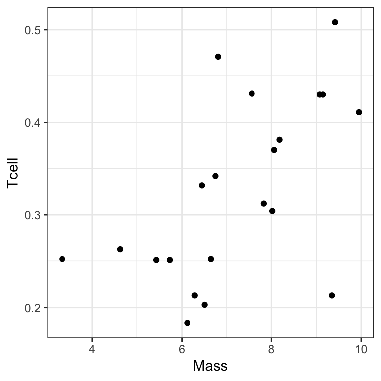
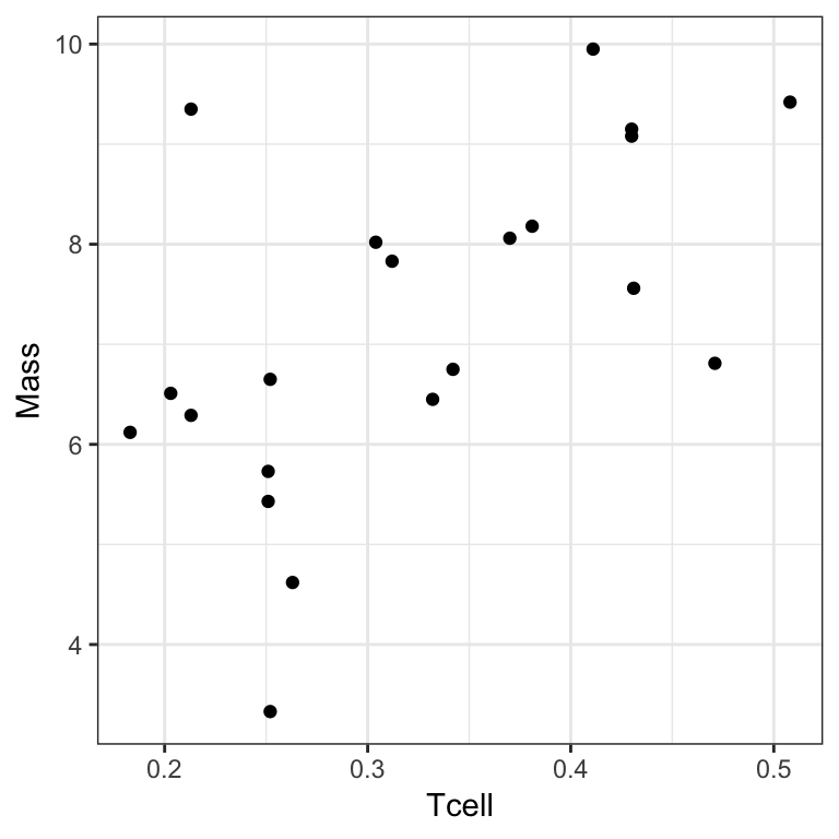
?ex0727Black wheatears are small birds in Spain and Morocco. Males of the species demonstrate an exaggerated sexual display by carrying many heavy stones to nesting cavities. This 35–gram bird transports, on average, 3.1 kg of stones per nesting season! Different males carry somewhat different sized stones, prompting a study on whether larger stones may be a signal of higher health status. Soler et al. calculated the average stone mass (g) carried by each of 21 male black wheatears, along with T-cell response measurements reflecting their immune systems’ strengths.
Your turn
There are two variables measured on 21 individual Black wheatears:
Massthe average mass of stones carried by the birdTcellthe T-cell response, a measure of the birds immune response
Discuss with your neighbour:
Which variable would you use as the response? Which variable is the explanatory variable? Why?
What parameter would you look at in your model to answer question of interest?
Interpretation of the parameters
Intercept, \(\beta_0\),
When the explanatory variable is zero, the mean response is \(\beta_0\).
Slope, \(\beta_1\),
An increase in the explanatory variable of one unit is associated with a change in mean response of \(\beta_1\).
(Careful with causal language…is it justified?)
But we don’t know \(\beta_0\) and \(\beta_1\)…
The least squares estimates
Find \(\hat{\beta_0}\) and \(\hat{\beta_1}\) so that the sum of squared residuals \[ \sum_{i=1}^{n} \left( y_i - (\hat{\beta_0} + \hat{\beta_1}x_i) \right)^2 \] is minimised.
Fitted values: \(\hat{y_i} = \hat{\beta_0} + \hat{\beta_1}x_i\)
Residuals: \(e_i = y_i - \hat{y_i}\)
We don’t require any properties of random variables to derive these estimates.
There are formulae for \(\hat{\beta_0}\) and \(\hat{\beta_1}\), how do you derive them?
Properties of the least squares estimates
Using the moment assumptions of \(\epsilon_i\), the least squares estimates can be shown to be unbiased. You can derive their variances, , , , but they depend on the unknown \(\sigma\).
An unbiased estimate of \(\sigma\) is \[ \hat{\sigma}^2 = \frac{ 1 }{n - 2} \sum_{i=1}^n e_i^2 \]
Intuition: \(\tfrac{1}{n} \sum_{i=1}^n e_i^2\) seems a reasonable place to start to estimate the variance of the errors, but this tends to underestimate the variance because we picked our estimates to make the sum of squared errors as small as possible.
In R
\[ \text{Mass}_i = \beta_0 + \beta_1 \text{Tcell}_i + \epsilon_i, \quad i = 1, \ldots, 21 \]
slr <- lm(Mass ~ Tcell, data = ex0727)summary(slr)
#>
#> Call:
#> lm(formula = Mass ~ Tcell, data = ex0727)
#>
#> Residuals:
#> Min 1Q Median 3Q Max
#> -3.1429 -0.7327 0.3448 0.7472 3.2736
#>
#> Coefficients:
#> Estimate Std. Error t value Pr(>|t|)
#> (Intercept) 3.911 1.112 3.517 0.00230 **
#> Tcell 10.165 3.296 3.084 0.00611 **
#> ---
#> Signif. codes: 0 '***' 0.001 '**' 0.01 '*' 0.05 '.' 0.1 ' ' 1
#>
#> Residual standard error: 1.426 on 19 degrees of freedom
#> Multiple R-squared: 0.3336, Adjusted R-squared: 0.2986
#> F-statistic: 9.513 on 1 and 19 DF, p-value: 0.006105