Goals:
- Lasso and ridge regression
- Sensitivity of model selection to transformations
library(tidyverse)Lasso and ridge regression
Work through code from Faraway 11.3 and 11.4
Meat fat content example from model selection examples in class:
data(meatspec, package = "faraway")
# Faraway takes the first 172 obs as training
# you shouldn't generally do that without careful
# thought
ind <- 1:172
trainmeat <- meatspec[ind, ]
testmeat <- meatspec[-ind, ]

# center all columns of x for ridge and lasso
x <- scale(meatspec[, -101], center = T, scale = F)
y <- meatspec[, 101]

testx <- x[-ind, ]
testy <- y[-ind]
trainx <- x[ind, ]
trainy <- y[ind]
rmse <- function(x,y) sqrt(mean((x-y)^2))fit_all <- lm(fat ~ ., data = trainmeat)
(rmse_all <- rmse(testmeat$fat, predict(fit_all, newdata = testmeat)))## [1] 3.814Recall that a model with all predictors, had an estimated root mean square prediction error of about 3.81.
fit_best <- lm(fat ~ V1+V17+V19+V20+V21+V24+V31+V35+V37+V39+V40+V41+V44+V47+V48+
    V51+V53+V57,
  data = trainmeat)
(rmse_best <- rmse(testmeat$fat, predict(fit_best, newdata = testmeat)))
## [1] 1.837097We also found some smaller models on Monday with smaller error, e.g., 1.84.
Ridge regression
Estimating the coefficients for a sequence of tuning parameters:
library(MASS)
rgmod <- lm.ridge(I(trainy - mean(trainy)) ~ trainx,
                  lambda = seq(0, 5e-8, 1e-9))

matplot(rgmod$lambda, coef(rgmod), type = "l",
  xlab = expression(lambda),
  ylab = expression(hat(beta)), col = 1)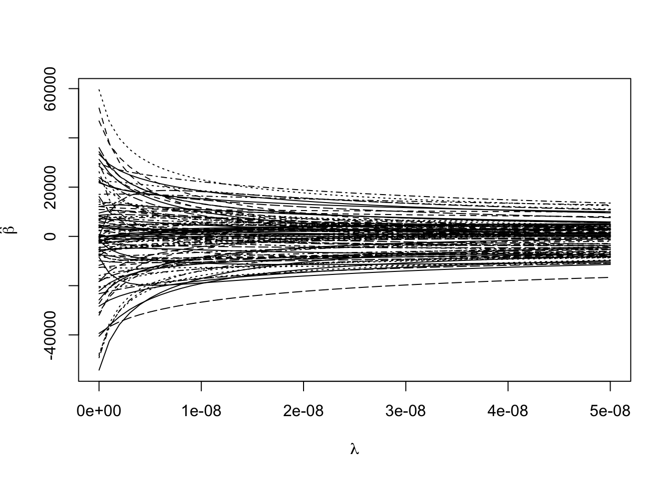
Choosing one tuning parameter:
(min_gcv <- which.min(rgmod$GCV))## 1.8e-08
## 19matplot(rgmod$lambda, coef(rgmod), type = "l",
xlab = expression(lambda),
ylab = expression(hat(beta)), col = 1)
abline(v = rgmod$lambda[min_gcv])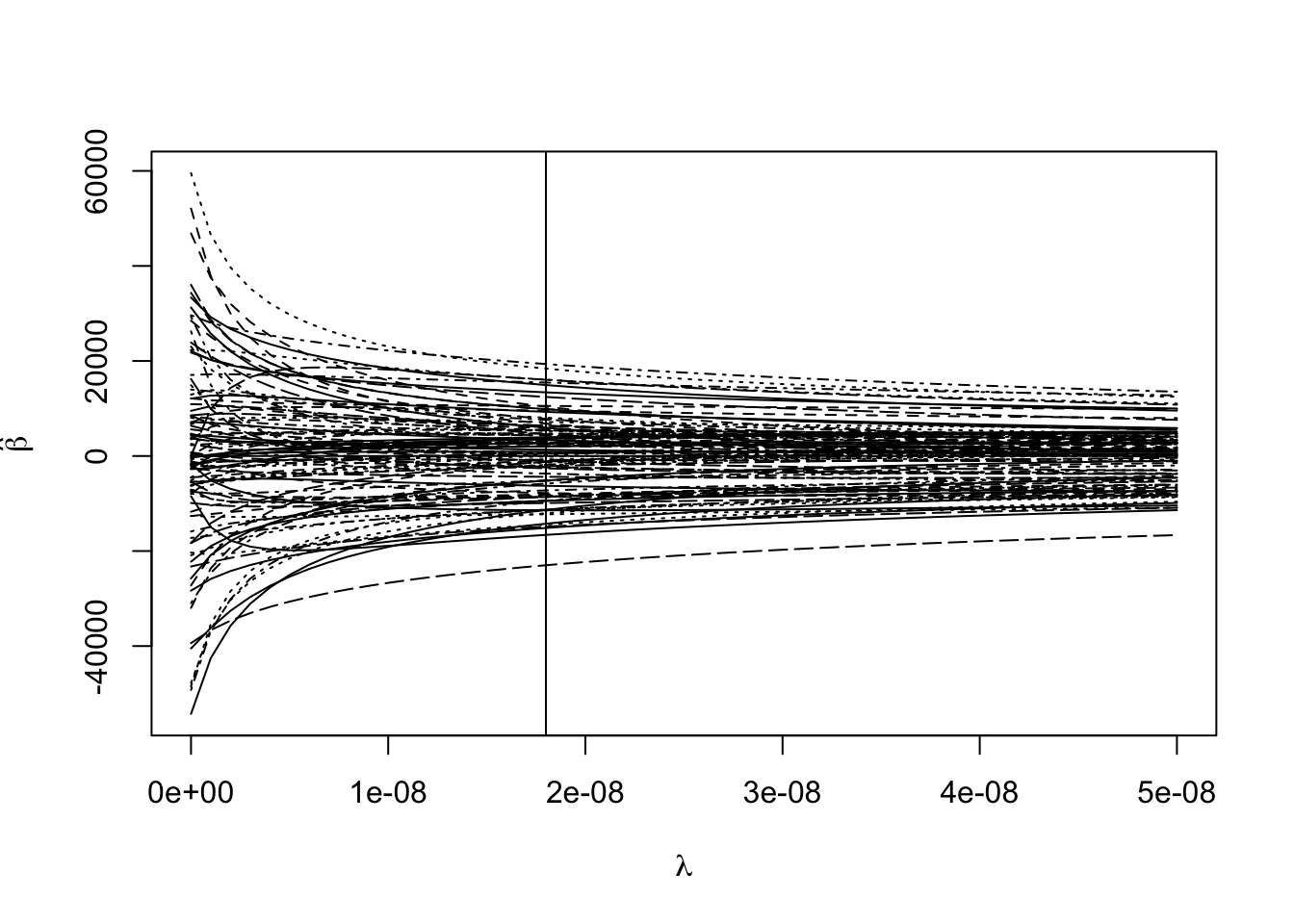
Evaluating the predictive accuracy:
ypred <- scale(trainx,
               center = F,
               scale = rgmod$scales) %*% # scale covariates
  rgmod$coef[, min_gcv] + # multiply by estimated coefficients
  mean(trainy) # add back mean (since response was centered)

rmse(ypred, trainy)
## [1] 0.8159824ypred <- scale(testx,
center = F,
scale = rgmod$scales) %*% # scale covariates
rgmod$coef[, min_gcv] + # multiply by estimated coefficients
mean(trainy) # add back mean (since response was centered)
rmse(ypred, testy)## [1] 4.067914One particularly bad prediction (looks OK to me, why does Faraway get something different?:
c(ypred[13], testmeat$fat[13])## [1] 11.32387 34.80000rmse(ypred[-13], testmeat$fat[-13])## [1] 1.954433cbind(ypred, testy)## testy
## 173 48.047247 47.7
## 174 23.143626 25.5
## 175 8.944386 10.6
## 176 3.461404 2.0
## 177 6.141724 4.7
## 178 6.741146 6.8
## 179 10.116475 8.6
## 180 11.781558 11.2
## 181 13.553112 13.8
## 182 14.937346 17.7
## 183 28.464430 23.3
## 184 24.774611 29.0
## 185 11.323870 34.8
## 186 46.180519 47.8
## 187 9.960860 11.1
## 188 4.791950 2.9
## 189 9.148401 4.8
## 190 5.900053 5.6
## 191 6.465477 6.2
## 192 6.794227 6.4
## 193 6.004676 6.8
## 194 6.815092 7.1
## 195 7.820161 7.3
## 196 8.016253 7.9
## 197 10.328492 9.2
## 198 9.358988 10.1
## 199 11.897665 10.7
## 200 7.628819 11.2
## 201 11.506780 12.5
## 202 14.621129 14.3
## 203 11.126646 16.0
## 204 16.681274 17.0
## 205 16.686706 18.1
## 206 20.448977 19.4
## 207 23.345195 24.8
## 208 26.978289 27.2
## 209 29.363296 28.4
## 210 29.227825 29.2
## 211 29.045001 31.3
## 212 31.692496 33.8
## 213 37.691766 35.5
## 214 41.439211 42.5
## 215 46.180519 47.8which.max(abs(ypred - testy))## [1] 13rmse(ypred[-13], testy[-13])## [1] 1.954433Lasso
library(lars)Example with a smaller set of predictors (the state life expectancy data from last week)
Estimating the coefficients for a sequence of tuning parameters:
statedata <- data.frame(state.x77, row.names = state.abb)
lmod <- lars(as.matrix(statedata[, -4]), statedata$Life)
Choosing one tuning parameter:
plot(lmod)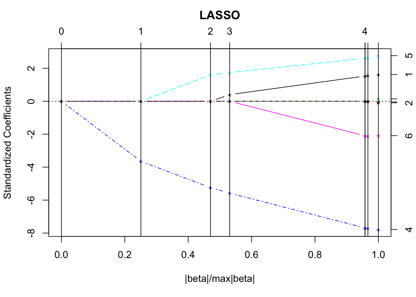
set.seed(123)
cvlmod <- cv.lars(as.matrix(statedata[, -4]), statedata$Life)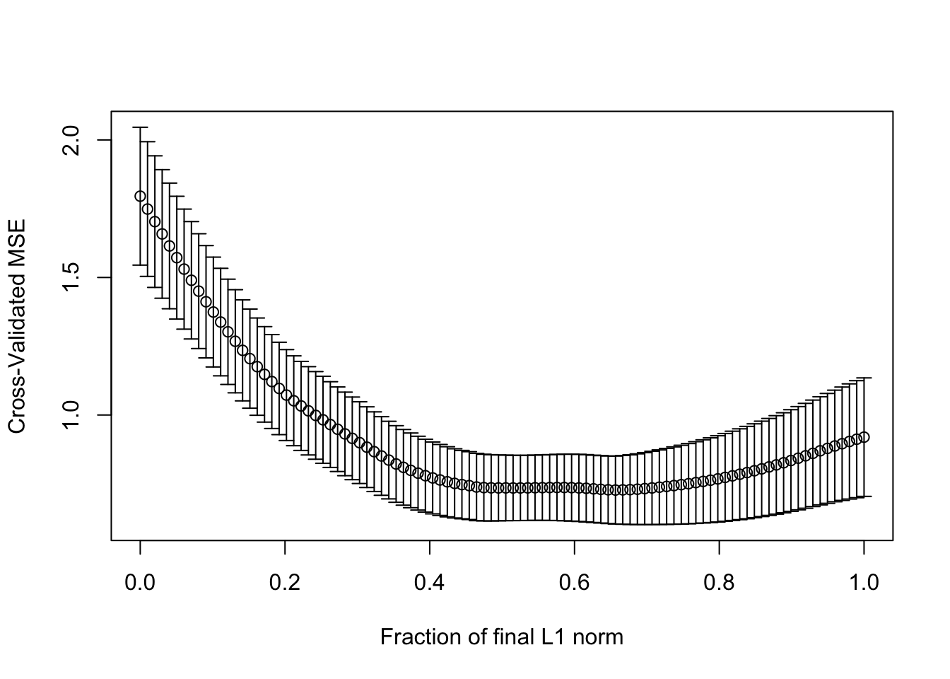
(s <- cvlmod$index[which.min(cvlmod$cv)])## [1] 0.6565657Compare the coefficients in the lasso model:
predict(lmod, s = s, type = "coef", mode = "fraction")$coef## Population Income Illiteracy Murder HS.Grad
## 2.345262e-05 0.000000e+00 0.000000e+00 -2.398786e-01 3.528871e-02
## Frost Area
## -1.694932e-03 0.000000e+00to those from the least squares fit:
coef(lm(Life.Exp ~ Population + Murder + HS.Grad + Frost, statedata))## (Intercept) Population Murder HS.Grad Frost
## 7.102713e+01 5.013998e-05 -3.001488e-01 4.658225e-02 -5.943290e-03Back to the meat fat example
Estimating the coefficients for a sequence of tuning parameters:
lassomod <- lars(trainx, trainy)Choosing one tuning parameter:
set.seed(123)
cvout <- cv.lars(trainx, trainy)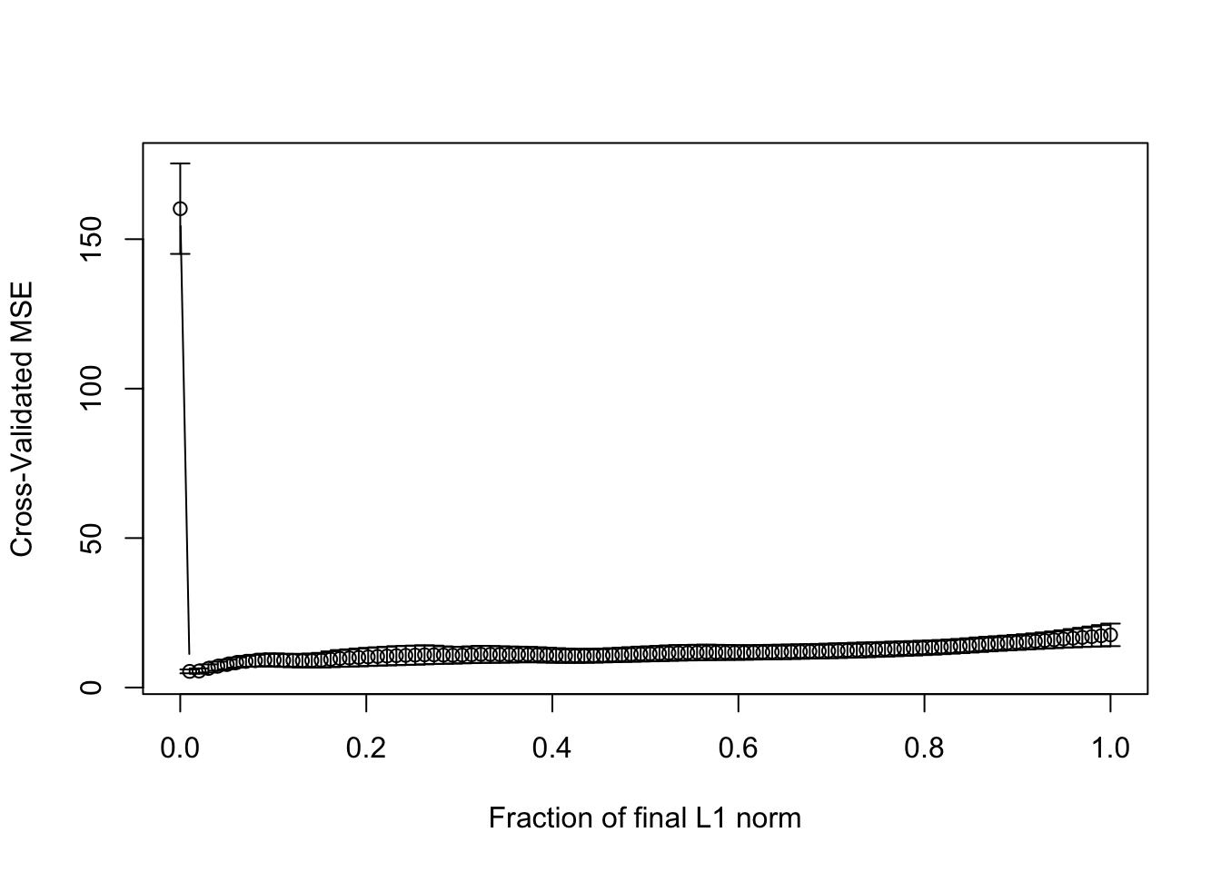
(best_s <- cvout$index[which.min(cvout$cv)])## [1] 0.01010101Evaluating the predictive accuracy:
predlars <- predict(lassomod, testx, s = best_s, mode = "fraction")
rmse(testy, predlars$fit)
## [1] 2.132218Examing which coefficients are non-zero:
predlars <- predict(lassomod, s = best_s, type = "coef", mode = "fraction")
plot(predlars$coef, type = "h", ylab = "Coefficient")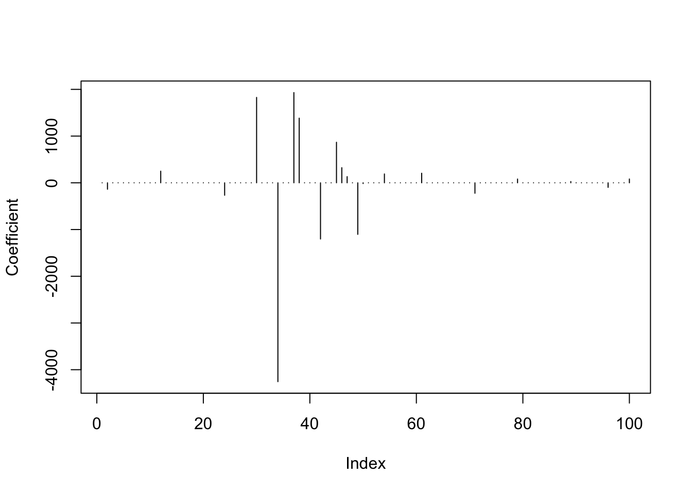
sum(predlars$coef != 0)## [1] 20Sensitivity of model selection
Work through code in Faraway 10.3
library(leaps)
source("http://stat552.cwick.co.nz/lecture/fortify-leaps.R")
In class we used regsubsets() to select variables to predict life expectancy from other state level data. In particular, imagine we use an exhaustive search and choose a model with the highest adjusted R-squared:
b <- regsubsets(Life.Exp ~ ., data = statedata)
rs <- summary(b)
rs$which[which.max(rs$adjr2),]
## (Intercept) Population Income Illiteracy Murder HS.Grad
## TRUE TRUE FALSE FALSE TRUE TRUE
## Frost Area
## TRUE FALSEIt’s possible this choice is sensitive both to indivudal points and transformations.
Alaska is unusual:
lmod <- lm(Life.Exp ~ ., data = statedata)
broom::augment(lmod) %>%
  arrange(desc(.hat))
## # A tibble: 50 x 16
## .rownames Life.Exp Population Income Illiteracy Murder HS.Grad Frost
## <chr> <dbl> <dbl> <dbl> <dbl> <dbl> <dbl> <dbl>
## 1 AK 69.3 365 6315 1.5 11.3 66.7 152
## 2 CA 71.7 21198 5114 1.1 10.3 62.6 20
## 3 HI 73.6 868 4963 1.9 6.2 61.9 0
## 4 NV 69.0 590 5149 0.5 11.5 65.2 188
## 5 NM 70.3 1144 3601 2.2 9.7 55.2 120
## 6 TX 70.9 12237 4188 2.2 12.2 47.4 35
## 7 NY 70.6 18076 4903 1.4 10.9 52.7 82
## 8 WA 71.7 3559 4864 0.6 4.3 63.5 32
## 9 OR 72.1 2284 4660 0.6 4.2 60 44
## 10 ND 72.8 637 5087 0.8 1.4 50.3 186
## # … with 40 more rows, and 8 more variables: Area <dbl>, .fitted <dbl>,
## # .se.fit <dbl>, .resid <dbl>, .hat <dbl>, .sigma <dbl>, .cooksd <dbl>,
## # .std.resid <dbl>Without it, the model selected changes:
b <- regsubsets(Life.Exp ~ ., data = statedata, subset = (state.abb != "AK"))
rs <- summary(b)
rs$which[which.max(rs$adjr2),]
## (Intercept) Population Income Illiteracy Murder HS.Grad
## TRUE TRUE FALSE FALSE TRUE TRUE
## Frost Area
## TRUE TRUENotice Area and Population might benefit from a transform:
stripchart(data.frame(scale(statedata)), method = "jitter", las = 2, vertical = TRUE)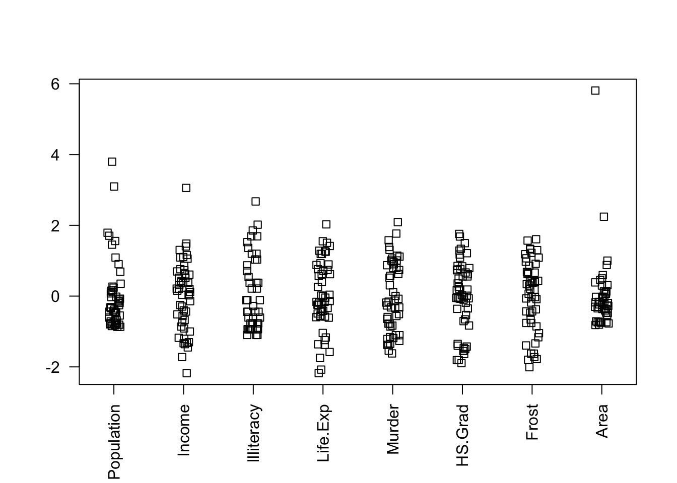
If we transform them, the selected model changes:
b <- regsubsets(Life.Exp ~ log(Population) + Income + Illiteracy + Murder + HS.Grad + Frost + log(Area), statedata)
rs <- summary(b)
rs$which[which.max(rs$adjr), ]
## (Intercept) log(Population) Income Illiteracy
## TRUE TRUE FALSE FALSE
## Murder HS.Grad Frost log(Area)
## TRUE TRUE TRUE FALSE