library(faraway)
library(tidyverse)
The code in today’s lab comes straight from Chapter 3 in Linear Models with R with only minor edits that I think improve clarity.
Preliminaries
Brief review of for loops
An example of a for loop in R:
n_sims <- 10
output <- numeric(n_sims)
for (i in 1:n_sims){
  output[i] <- mean(rnorm(20))
}
output
## [1] -0.21798434 -0.16131401 0.50563841 -0.25441329 0.14596754
## [6] 0.18129472 -0.14947953 0.02673052 0.09009637 -0.12237762TA to remind you about parts of a for loop:
- Output
- Sequence
- Body
There are alternatives to for loops that remove all the repetitive book-keeping parts and let you focus on what is being done rather than how it is being done, for example the map() functions in the purrr package. We won’t use them here, because when you see these statistical methods first, I think the for loop syntax more closely matches the textual description of what is happening (at least how Faraway describes it).
The sample() function
Used in two ways (in Chapter 3 in Faraway):
To randomly permute a set of values:
sample(1:5)## [1] 3 4 2 1 5sample(c("a", "b", "c"))## [1] "a" "c" "b"With no further arguments,
sample()will randomly reorder the vector you give it.To sample with replacement from a set of numbers, add
replace = TRUE:sample(1:5, replace = TRUE)## [1] 4 3 3 3 5sample(c("a", "b", "c"), replace = TRUE)## [1] "a" "c" "c"
In both cases we are omitting the size argument, which by default is the same as the length of the input vector.
Bootstrap confidence intervals
Overall idea: To understand the sampling distribution of a parameter estimate, generate data that approximate what repeated experiments/samples would look like.
Procedure From Faraway (Model based bootstrap)
Repeat many times:
- Generate \(\epsilon^*\) by sampling with replacement from the residuals, \(e_1, \ldots, e_n\).
- Form \(y^* = X\hat{\beta} + \epsilon^*\).
- Compute \(\hat{\beta}^*\) from \((X, y^*)\).
Examine distribution of parameter estimates generated by bootstrap to make inferences on true parameter value.
Setup
Model based bootstrapping requires us to assume a specific model form, fit it:
lmod <- lm(Species ~ Area + Elevation + Nearest + Scruz + Adjacent,
  data = gala)
And retain the fitted values and residuals:
resids <- residuals(lmod)
preds <- fitted(lmod)
A single bootstrap sample
A single bootstrap dataset is constructed by adding the fitted values (i.e. \(X\hat{\beta}\)), and bootstrapped errors (a sample with replacement from the residuals):
# bootstrapped errors
(errors <- sample(resids, replace = TRUE))
## Eden Isabela Espanola Champion SanCristobal
## -20.314202 -39.403558 49.343513 14.635734 73.048122
## Pinzon Isabela SantaCruz Enderby Gardner1
## -42.475375 -39.403558 182.583587 -28.785943 62.033276
## Pinzon Champion Bartolome Pinta SantaFe
## -42.475375 14.635734 38.273154 -111.679486 -23.376486
## Pinta Bartolome Genovesa Isabela Espanola
## -111.679486 38.273154 40.497176 -39.403558 49.343513
## Pinzon Rabida Baltra Coamano SantaCruz
## -42.475375 -5.553122 -58.725946 38.383916 182.583587
## Darwin Caldwell Pinta Tortuga Seymour
## 19.018992 -26.330659 -111.679486 -36.935732 -5.805095# bootstrapped response
preds + errors## Baltra Bartolome Caldwell Champion Coamano
## 96.4117443 -46.6767121 78.6741729 25.0000000 36.6642065
## Daphne.Major Daphne.Minor Darwin Eden Enderby
## 0.6123302 -5.4838900 173.5645950 -0.4717408 92.8192184
## Espanola Fernandina Gardner1 Gardner2 Genovesa
## 5.1811115 111.6253322 34.2398785 -47.0456905 -23.8736612
## Isabela Marchena Onslow Pinta Pinzon
## 274.7240716 126.9676948 44.5344083 176.2759284 199.8188885
## Las.Plazas Rabida SanCristobal SanSalvador SantaCruz
## -7.3995684 70.0000000 148.2259319 316.0602339 444.0000000
## SantaFe SantaMaria Seymour Tortuga Wolf
## 104.3954776 169.2859692 -61.8743916 16.0000000 20.8954789In this example our model involves multiple terms so it’s a little hard to visualise. But here are the original fitted values (blue open dots) along with the a bootstrapped set of response values (black filled dots) against one of the predictors, Elevation:
ggplot(gala, aes(Elevation, preds)) +
  geom_point(color =  "#377EB8", shape = 21) +
  geom_point(aes(y = preds + errors), color = "black")+
  ylim(c(-200, 500))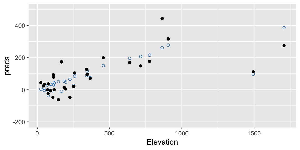
Here’s another one:
errors <- sample(resids, replace = TRUE)
ggplot(gala, aes(Elevation, preds)) +
  geom_point(color =  "#377EB8", shape = 21) +
  geom_point(aes(y = preds + errors), color = "black") +
  ylim(c(-200, 500))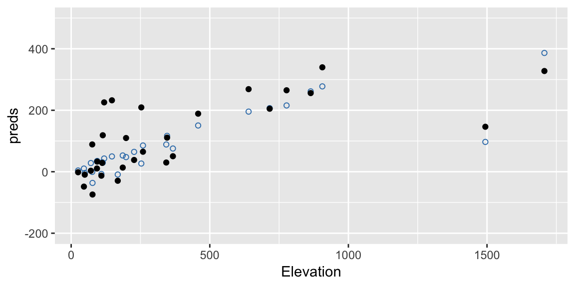
Notice this process retains the structure implied by the fitted model. So, if our model has a large effect due to Elevation, we should maintain that effect in our bootstrap samples.
Repeating many times
We can repeat this process many times each time fitting the model and retaining the estimated coefficients:
nb <- 4000
coefmat <- matrix(NA, nrow = nb, ncol = 6)
colnames(coefmat) <- names(coef(lmod))
for (i in 1:nb){
  booty <- preds + sample(resids, replace = TRUE)
  bmod <- update(lmod, booty ~ .)
  coefmat[i, ] <- coef(bmod)
}
Then using these many estimated coefficients we can construct confidnce intervals using the percentile method:
(cis <- apply(coefmat, 2, quantile, probs = c(0.025, 0.975)))## (Intercept) Area Elevation Nearest Scruz Adjacent
## 2.5% -25.04466 -0.06304558 0.2259949 -1.683388 -0.6046124 -0.10553011
## 97.5% 41.41317 0.02103163 0.4198246 2.139087 0.1760862 -0.03806448Or create density plots on individual parameters:
coefmat <- as_tibble(coefmat)
cis <- as_tibble(cis)

ggplot(coefmat, aes(x = Area)) +
  geom_density() +
  geom_vline(aes(xintercept = Area), data = cis, linetype = "dashed",
    color = "grey20") +
  labs(title =
      expression(paste("Bootstrap estimate of the sampling distribution for ", hat(beta)[Area])))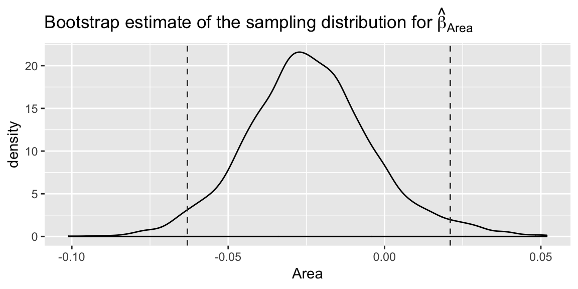
Permutation tests
Overall idea: To understand the null distribution of a test statistic, approximate what repeated experiments/samples would look like, if the null hypothesis was true.
Procedure
Repeat many times:
- Generate \((X^*, y^*)\) by permutation, in a way suggested by the null hypothesis.
- Compute test statistic \(T(X^*, y^*)\).
Compare observed test statistic to the distribution of test statistics generated by permutation, to conduct a hypthothesis test.
An overall F-test example
Faraways chooses an example with a not too small overall F-test p-value (I’ve given this model object a different name to Faraway to emphasize this is not the same model as lmod above):
lmod_small <- lm(Species ~ Nearest + Scruz, data = gala)
lms <- summary(lmod_small)
The overall F-test statistic is available:
lms$fstatistic## value numdf dendf
## 0.6019558 2.0000000 27.0000000which we can use to find the corresponding p-value:
1 - pf(lms$fstatistic[1], lms$fstatistic[2], lms$fstatistic[3])## value
## 0.5549255This p-value is based on our assumption of Normal errors. We’ll save the statistic for later:
obs_fstat <- lms$fstat[1]The permutation approach attempts to find the null distribution of this test statistic without relying on any distributional assumptions. The null hypthothesis in this overall F-test, is that none of the explanatory variables impact our response. If this was the case, the response value we see for a particular island shouldn’t depend on its attributes. We should have been just as likely to see 58 species on Bartolome and 31 species on Baltra instead of the other way around. In fact, any permutation of the response values assigned to islands should have been equally likely to occur.
(Notice this feels a little awkward with observational data. It is generally much easier to justify a permutation approach in a randomized experiment, where the treatment variables were actually assigned to units at random.)
A single permutation
To generate a null distribution of the test statistic we consider permutations of the response variable.
permuted_species <- sample(gala$Species)Again its hard to visualise becasue we have a few variables involved, but take a look at this permuted response (black filled points) against Elevation:
ggplot(gala, aes(Elevation, Species)) +
  geom_point(color = "#377EB8", shape = 21) +
  geom_point(aes(y = permuted_species), color = "black") +
  ylim(c(-200, 500))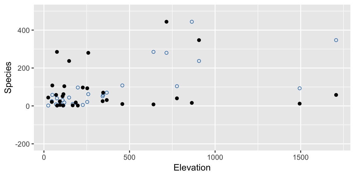
Notice that a key difference between this and the bootstrap approach is that we break relationships here. In the original data there was a strong relationship between Elevation and Species, but under the null hypothesis there isn’t, and our permutated data reflects this.
To get a test-statistic from this data, we fit the model of interest and extract the F-statistic:
lm_permutation <- lm(permuted_species ~ Nearest + Scruz, data = gala)
summary(lm_permutation)$fstat[1]
## value
## 7.434452This is an example of one test statistic generated under the null hypothesis, to conduct a test we need a whole lot of them.
Scaling up
nperms <- 4000
fstats <- numeric(nperms)
for (i in 1:nperms){
  lmods <- lm(sample(Species) ~ Nearest + Scruz, data = gala)
  fstats[i] <- summary(lmods)$fstat[1]
}
These statistics then form our null distribution:
ggplot(mapping = aes(x = fstats)) +
  geom_density() +
  geom_vline(aes(xintercept = obs_fstat), linetype = "dashed",
    color = "grey20") +
  labs(title = "Permutation based null distribution for the overall F-statistic",
    xlab = "F-statistic")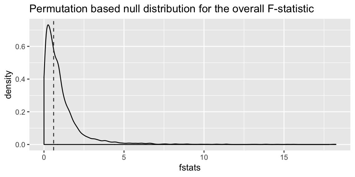
And to get a p-value, we find the proportion of test statistics generated under the null hypothesis that are more extreme than that observed:
mean(fstats > obs_fstat)## [1] 0.5565In this case, pretty close to the p-value derived using the Normal assumptions.
An individual parameter example
You can also use a permuation approach to test individual parameter estimates in a regression. Now, since the null hypothesis is only about one parameter, after accounting for the effects of the other variables, we only permute values of the explanatory varibale of interest.
For example, in lmod_small we might ask only about the parameter on Scruz, \(\beta_{\text{Scruz}}\). For the null hypothesis \(\beta_{\text{Scruz}} = 0\), the Normal based inference gives us a p-value of 0.28:
summary(lmod_small)$coef## Estimate Std. Error t value Pr(>|t|)
## (Intercept) 98.4765494 28.3561013 3.472852 0.001751461
## Nearest 1.1792236 1.9184475 0.614676 0.543914527
## Scruz -0.4406401 0.4025312 -1.094673 0.283329519We’ll still the t-statistic as our test statistic, so we’ll keep the value from the observed data:
obs_tstat <- summary(lmod_small)$coef[3, 3]But now we’ll use permutation to find a null distribution rather than relying on theory and comparing it to a Student’s t-distribution.
tstats <- numeric(nperms)
for (i in 1:nperms){
  lmods <- lm(Species ~ Nearest + sample(Scruz), data = gala)
  tstats[i] <- summary(lmods)$coef[3, 3]
}
Here’s the resulting null distribution, with the t-distribution that the Normal assumption would lead to overlaid:
ggplot(mapping = aes(x = tstats)) +
  geom_density() +
  geom_vline(aes(xintercept = obs_tstat), linetype = "dashed",
    color = "grey20") +
  stat_function(fun = dt, args = list(df = lmod_small$df.residual),
    color= "grey50")+
  labs(title = expression(
    paste("Permutation based null distribution for the t-statistic, ", beta[Scruz]==0)),
    xlab = "t-statistic")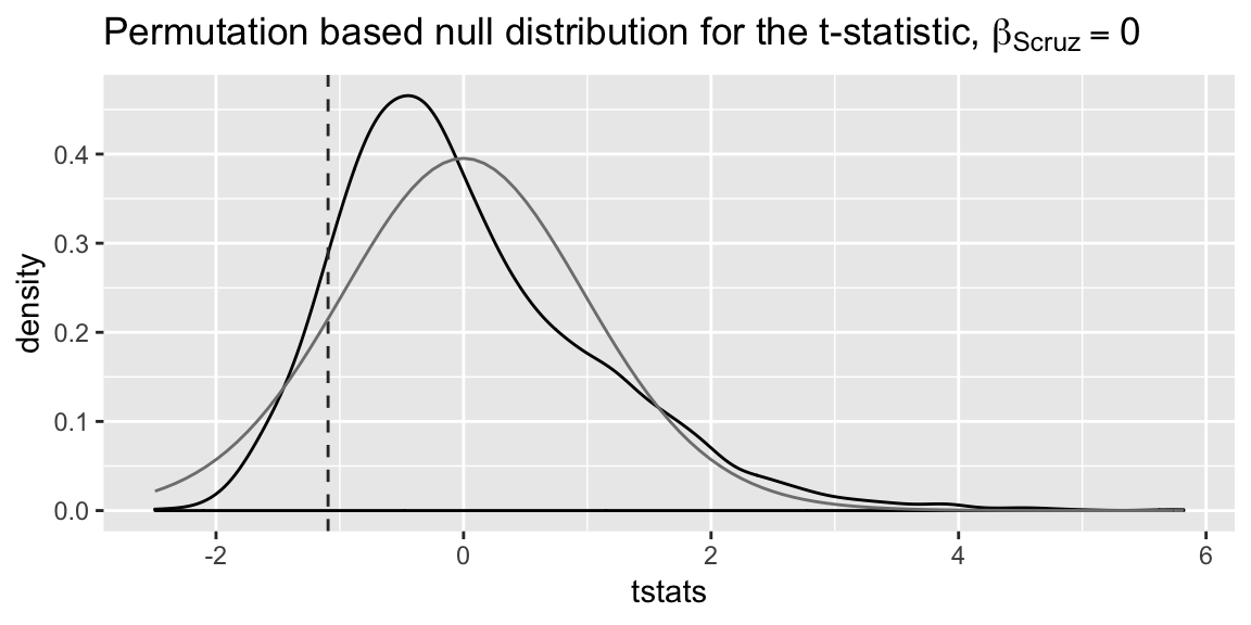
Notice the null distribution based on the permutation test doesn’t seem that close to the t-distribution. However, the p-value isn’t particularly different in this case:
mean(abs(tstats) > abs(obs_tstat))## [1] 0.26375