Today
- Another view of F-tests
- Confidence intervals for single parameters
- Confidence intervals for linear combinations of parameters
- Confidence intervals for parameters jointly
Last time…
Certain hypotheses of interest can be set up as competing models. A full model and a simpler model (nested in the full model). A.K.A testing models.
Identify the models of interest. Fit both. Check fit of full model. Find F-statistic, and answer questions of interest.
Another way to set up F-tests A.K.A testing linear parametric functions
Assuming the regression model: \[ Y = X\beta + \epsilon, \quad \epsilon \sim N(0, \sigma^2 I) \] Consider the hypotheses: \[ \begin{aligned} H_0: K^T \beta = m \\ H_1: K^T \beta \ne m \end{aligned} \] where \(K_{k \times p}\) matrix with rank(K) = k.
Then under the null hypothesis, \[ F = \frac{\left((K^T\beta - m)^T \left(K^T(X^TX)^{-1}K \right)^{-1} (K^T\beta - m)\right)/k}{\text{RSS}/(n-p)} \sim F_{k, n-p} \]
(Don’t memorise for ST552, maybe for comps)
You get the same answer
This alternative is equivalent to the model testing setup we considered. Every null hypothesis of the form \(K^T \beta = m\) is comparing a full and reduced model and vice versa.
For example, consider \[ K = \left(\begin{matrix} 0 \\ \vdots \\ 0 \\ 1\\ 0 \\ \vdots \\ 0 \end{matrix}\right), \quad m = 0 \hspace{3cm} \] where the 1 in \(K\) occurs in the \(i\)th row.
What is the null hypothesis being tested?
Your turn
What are \(K\) and \(m\) for exercises 1 and 5 from the handout from last time? HW#4
Confidence intervals for individual \(\beta_j\)
The t-test for an individual parameter can be flipped around to give \(100(1 - \alpha)\%\) confidence intervals of the form
\[ \hat{\beta_j} \pm t^{(\alpha/2)}_{n-p} \SE{\hat{\beta_j}} \]
(Remember \(\SE{\hat{\beta_j}}\) is coming from the diagonal entry of the estimated variance-covariance matrix.)
Coagulation times
Dataset comes from a study of blood coagulation times. 24 animals were randomly assigned to four different diets and the samples were taken in a random order.
Consider the model: \[ \begin{aligned} \text{Coagulation time (s)}_i &= \beta_0 + \beta_1 1\{\text{Diet B}\}_i \\ &+ \beta_2 1\{\text{Diet C}\}_i + \beta_3 1\{\text{Diet D}\}_i + \epsilon_i \end{aligned} \]
Coagulation
data(coagulation, package = "faraway")
ggplot(coagulation, aes(diet, coag)) +
  geom_dotplot(binaxis = "y",  binwidth = 1)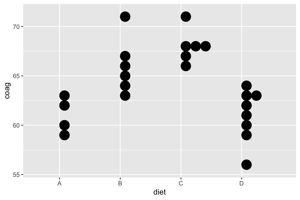
Your turn: cont.
fit <- lm(coag ~ diet, data = coagulation)
broom::tidy(fit) %>%
knitr::kable(digits = 2)| term | estimate | std.error | statistic | p.value |
|---|---|---|---|---|
| (Intercept) | 61 | 1.18 | 51.55 | 0 |
| dietB | 5 | 1.53 | 3.27 | 0 |
| dietC | 7 | 1.53 | 4.58 | 0 |
| dietD | 0 | 1.45 | 0.00 | 1 |
Find a 95% CI for \(\beta_0\)?
\(t_{n-p}^{(0.975)}= t_{20}^{(0.975)} = 2.09\)
Your turn: cont.
In R:
broom::tidy(fit, conf.int = TRUE)
# OR
(cis <- confint(fit))
Confidence intervals for linear combinations of parameters of \(\beta_j\)
Similarly, confidence intervals for a linear combination of the parameters, \(c^T\beta\) where \(c_{p\times 1}\), can be formed with \[ c^T\hat{\beta} \pm t^{(\alpha/2)}_{n-p} \sqrt{\hat{\sigma}^2 c^T(X^TX)^{-1}c} \]
Your turn
With the coagulation example \[
\begin{aligned}
\text{Coagulation time (s)}_i &= \beta_0 + \beta_1 1\{\text{Diet B}\}_i \\
&+ \beta_2 1\{\text{Diet C}\}_i + \beta_3 1\{\text{Diet D}\}_i + \epsilon_i
\end{aligned}
\]
What is \(c\) for the linear combination \(\beta_0 - \beta_1\)?
Find \(c^T(X^TX)^{-1}c\).
X <- model.matrix(fit)
round(solve(t(X) %*% X), 2)
## (Intercept) dietB dietC dietD
## (Intercept) 0.25 -0.25 -0.25 -0.25
## dietB -0.25 0.42 0.25 0.25
## dietC -0.25 0.25 0.42 0.25
## dietD -0.25 0.25 0.25 0.37Joint confidence regions
A joint \(100(1-\alpha)\%\) confidence for the vector \(\beta\) can be formed using, \[ (\hat{\beta} - \beta)^TX^TX(\hat{\beta} - \beta) \le p \hat{\sigma}^2 F^{(\alpha)}_{p, n-p} \] and results in \(p\)-dimensional ellipsoids (very hard to visualise, but essential for communicating joint uncertainty when the parameters are correlated).
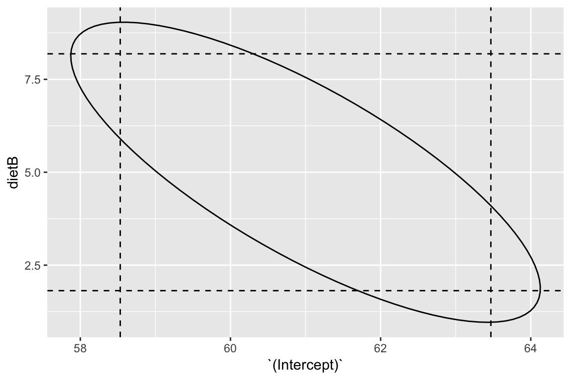
2D ellipsoid example: correlated estimates
For example, \((\beta_0, \beta_1)\) in
\[ \begin{aligned} \text{Coagulation time (s)}_i &= \beta_0 + \beta_1 1\{\text{Diet B}\}_i \\ &+ \beta_2 1\{\text{Diet C}\}_i + \beta_3 1\{\text{Diet D}\}_i + \epsilon_i \end{aligned} \]
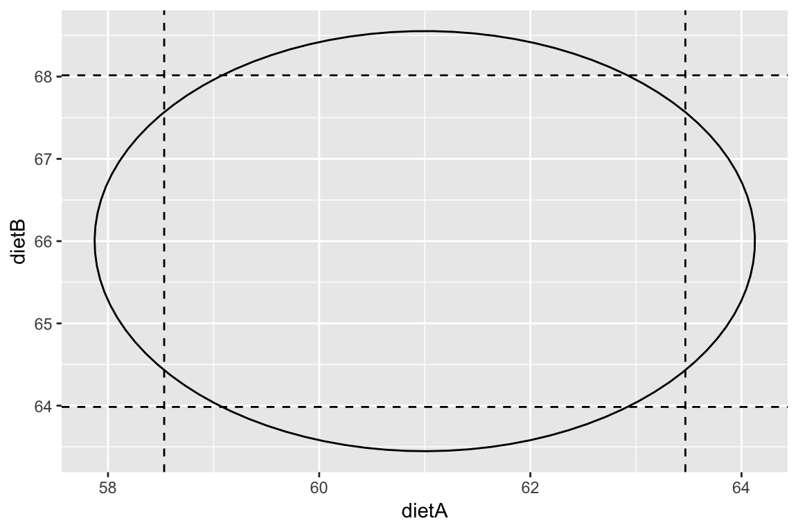
2D ellipsoid example: uncorrelated estimates
Compare to \(\gamma_0\) and \(\gamma_1\) in this parameterization: \[ \begin{aligned} \text{Coagulation time (s)}_i &= \gamma_0 1\{\text{Diet A}\}_i + \gamma_1 1\{\text{Diet B}\}_i \\ &+ \gamma_2 1\{\text{Diet C}\}_i + \gamma_3 1\{\text{Diet D}\}_i + \epsilon_i \end{aligned} \]
fit_nointercept <- lm(coag ~ diet - 1, data = coagulation)